Chapter 3: Build your AI Project with KNN and PyScript
This chapter focuses on the development of a simple website that uses PyScript, HTML, Python, Numpy and KNN. This is the main AI portion of the book and the project we are trying to complete and deploy to the web using GitHub. We previously described KNN as the K Nearest Neighbors algorithm. It is our first machine learning algorithm in this book series. KNN is a great algorithm to start your journey into the world of AI. It is simple enough, very useful, and can be coded from scratch efficiently using only a few lines of code with Python and Numpy.
Copyright and License
All rights reserved. No part of this work may be reproduced or transmitted in any form or by any means, without written permission of the copyright owner.
MIT License.
FTC and Amazon Disclaimer
This post/page/article includes Amazon Affiliate links to products. This site receives income if you purchase through these links.
This income helps support content such as this one.

So, what can KNN do? KNN is what is known as a machine learning algorithm for classification. If you recall, in chapter 1,
I gave a quick explanation of KNN using a vector space of different balls used in sports. I said that, in essence, KNN is used
for classification. We can imagine a space where you have many balls from different sports. Some are soccer balls, others are baseballs, others are
basketballs, tennis balls, etc. They are all floating in this space. Each ball is described by a specific set of characteristics called features.
These features can be for color, diameter, shape, number of lines or curves, etc. Some balls are smaller than others, etc. Some are greener than others.
The main idea is that similar balls in this vector space will be closer to each other based on these features. Imagine all the bigger balls on the top left
side of the space and all the smaller balls on the lower right side of the space as can be visualized in the figure below.
Now, when we add a new ball in this space, its features will force it to be closer to the balls that have similar features to it.
This number of features can be 2 or 3 or 10 or 784 or more. Our cubic space of balls in the figure only has 3 features or dimensions.
But there is no limit to the number of features or dimensions. The Iris dataset, for instance, would exist in a space of 4 dimensions.
Even though we can't visualize it, the coding and math holds.
Think of each feature as an axis in this space. If we view the space of balls in the figure, we immediately know what the ball is. But since AIs do not have eyes (yet),
they have to rely on other methods. In this case, KNN should solve this problem.
Look at the figure again. In the lower right hand corner there are 3 white baseball balls and one green tennis ball. And then there is an odd looking ball with the
shape of a baseball and the color of a tennis ball. What is it? That is what KNN tries to solve. Is this odd looking ball closer to the green tennis ball or the
baseball shaped balls? The values of the features are what help KNN to solve this problem.
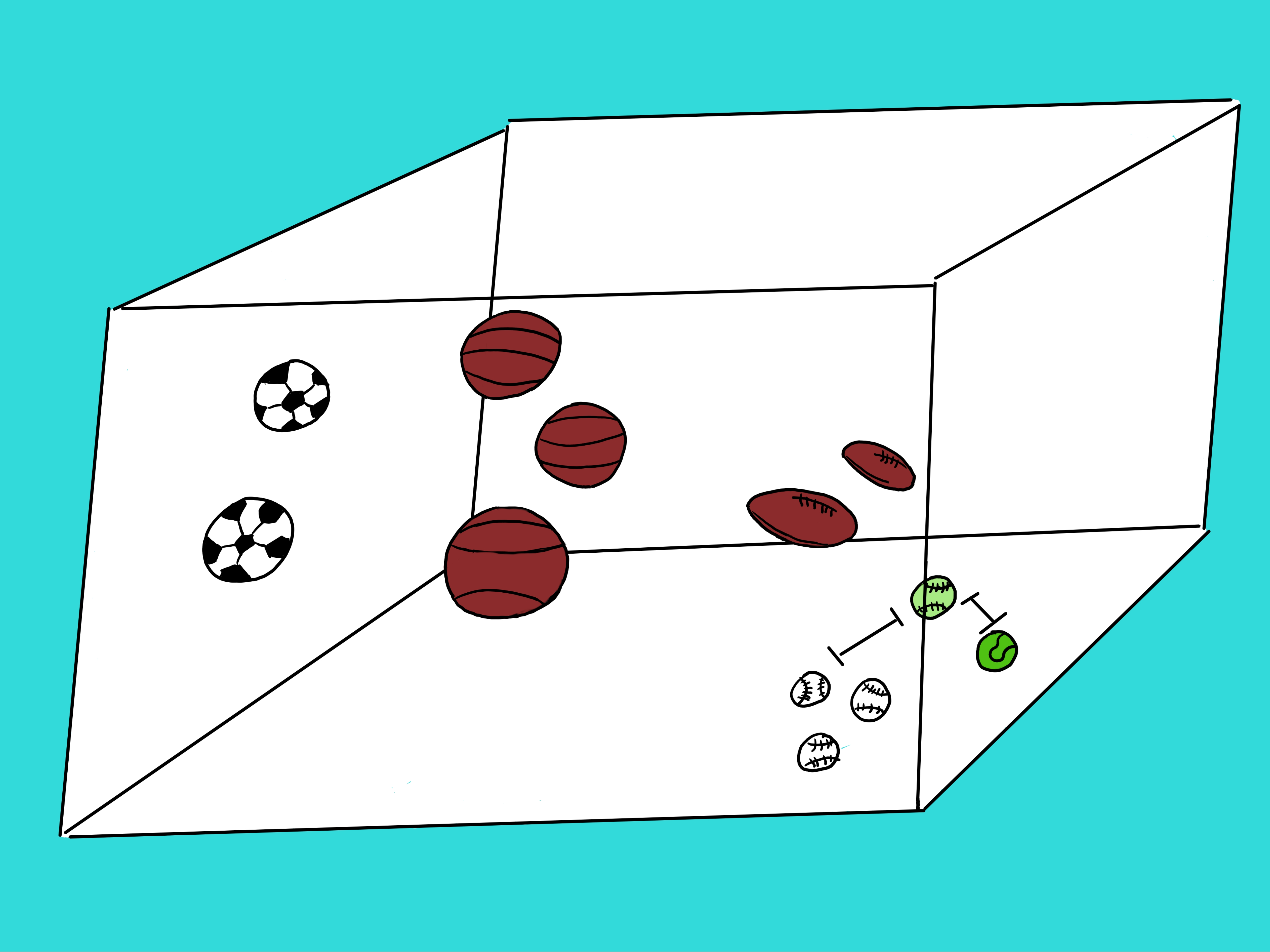
Basically, KNN will take a sample in question, say the green baseball, and measure the distance between it and all other balls in this space (i.e. the soccer balls,
basket balls, football balls, tennis balls, and baseballs). Once KNN calculates all the distances, it will rank then from lowest to highest distance.
Out of these ranked distances, it will select the top \textbf{k} distances and assign to the ball in question the majority class from the set containing just
the top "k" shortest distances. For the given example, if we selected a k=5 then the 5 closest balls to the ball in question (green baseball) would be 3
baseballs, 1 tennis ball, and one football. Since the majority is baseball, KNN would assign the class baseball to our ball in question. From the figure,
that would seem like the right answer. In the next sections, I will proceed to describe how to implement, test, and deploy our KNN machine learning model to the web.
In the next 2 sections, I will describe the KNN algorithm. The first of the 2 sections is the basic implementation of KNN. It involves building the model and running it.
Usually this is where you figure out the performance metric of your model. We will still run it on the browser and deploy it but it will not be a general use
App where we can add our inputs and do inference. Inference is a term used in AI which usually means prediction. The second of these 2 sections will do just that
and use what we learned in the first section to build our inference application. A lot will be the same but it will take data from text boxes and we will need to
make changes to execute this new functionality.
In summary, the next 2 sections cover:
- Basics to get KNN running
- A KNN app that you can use with user supplied data for Iris flower classification
Basics to get KNN running
As you may remember from the previous chapters, first we need to define the HTML code that encapsulates the PyScript code, which in turn, encapsulates our KNN algorithm implemented in Python and Numpy. The code in the next code listing should be familiar to you by now. Everything in the head section is similar to what we have previously described. The body section also includes the same \textbf{div} tags and the \textbf{button} we discussed in chapters 1 and 2.
In the next code listing we can see the previously discussed PyScript section denoted by
This section contains the previously discussed 3 items: the "div" with "mpl" id we have used before, the "config" section for libraries we want to use, and the
section where we write out actual Python and Numpy code.
In the next code listing, you can see all the code needed to run KNN. Wow! Pretty short right? This code splits our data into "train" and "test" sets. Then grabs every sample in the test set and compares it to every sample in the train set. As previously described, for each test sample, we get all distances between the test samples and all train samples. We then rank them and select the top "K" distances. Finally, we assign the majority class associated for the top 5 distances. That is it!
Okay, so I always like to see the big picture first. And that is what the previous code listing was for. Now we can proceed to break the code down into the various parts and describe what they are doing. In the next code listing we can see all the libraries needed for our KNN implementation. We have Numpy, Pandas, Pyodide, and Matplotlib. Numpy as you know by now is for all the math. Pandas is used in this project book to read in the data. Pyodide is intrinsic to PyScript and it is very important to run Python on the web. Matplotlib is not used in this project book but it is very important for AI research. You will be amazed in future project books by its capabilities for data visualization.
and
The next section in the code includes a function called the Euclidean distance as can be seen in the next code listing.
This is the function that measures the distance between 2 points in a vector space. These 2 point need to have the same size but the size can be of any dimension.
For instance, for our Iris data, every point has 4 features. So in the code the 2 points v1 and v2 would be of size 4 each. However, we could also have points
(samples) of many more dimensions. For instance, points with 100 features. So in this case v1 and v2 would both need to have size 100. But the cool thing is that
the function for distance calculation would still work. That is the power of Numpy.
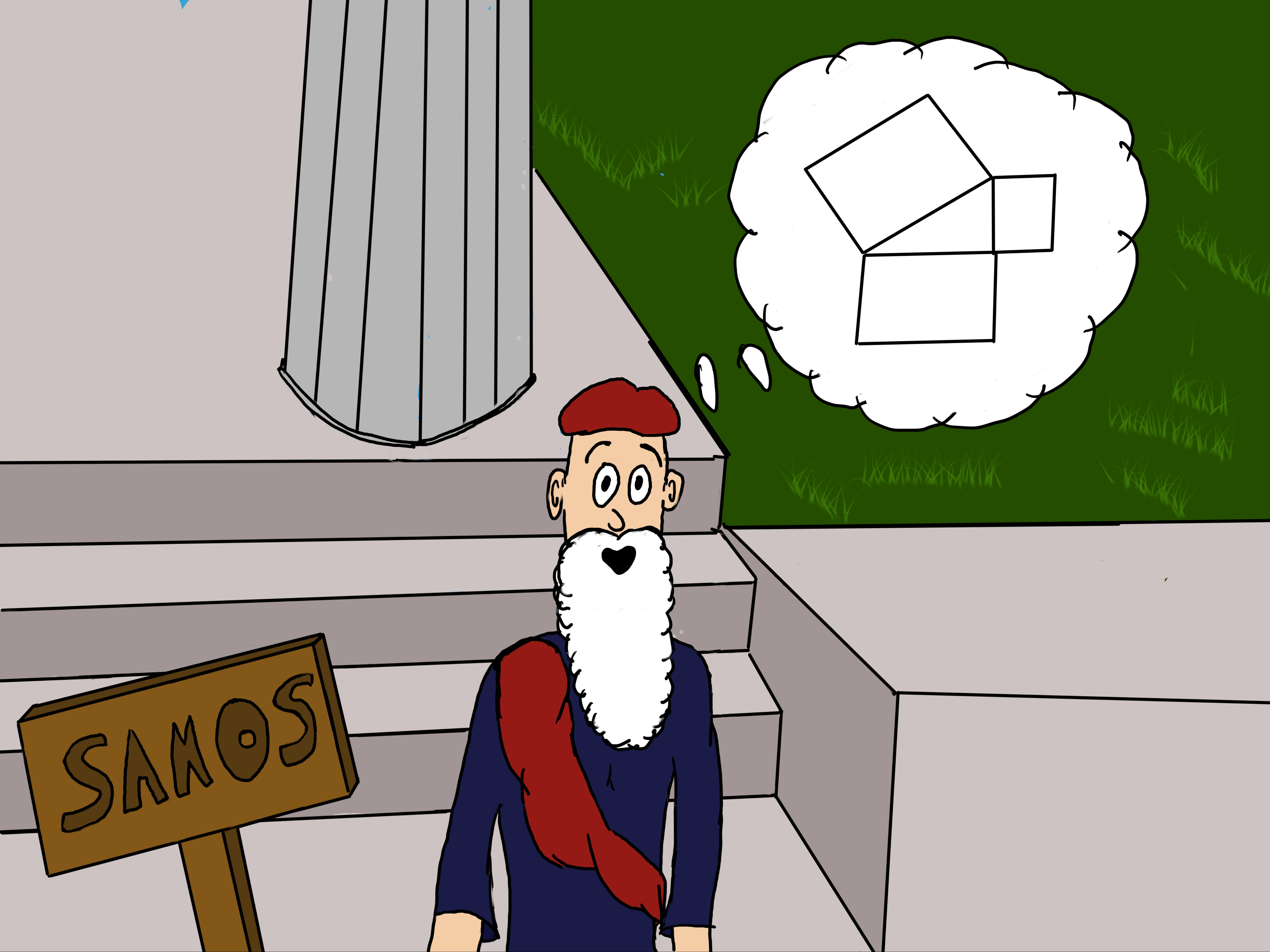
The name Euclidean distance comes from a Greek philosopher named Euclid. He is best known for putting together one of the earliest books on geometry.
The book was so good for its time that the type of mathematics it discussed became known as Euclidean geometry.
So, where does this magical Euclidean distance function come from? Would you believe that it is related to an idea one of the great Greek philosophers
(Pytagoras) is credited with? Pytagoras was before Euclid and is credited with coming up with the Pythagorean Theorem (bubble in the figure).
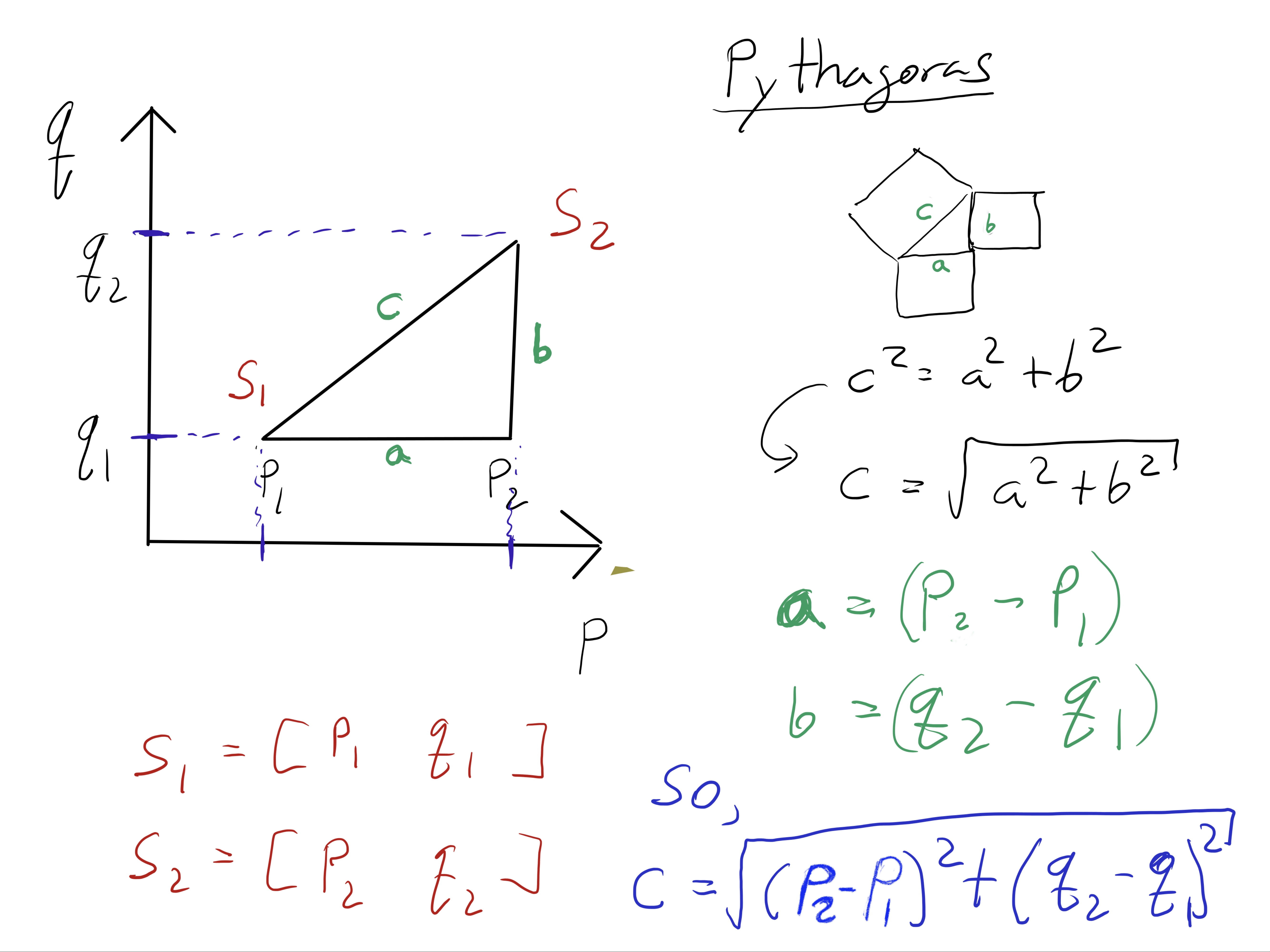
The theorem states that given a triangle (see figure below), the sum of the areas of the two squares on the legs (a and b in green) equals the area
of the square on the hypotenuse (c in green).
If you look closely at the figure below, you can see that I have written down the connection between Pythagoras' theorem, and the euclidean function we used in our code.
Now, with some of the math history out of the way, let us continue with our code description. In the next code listing we can see the KNN \textbf{predict} function. Actually, the \textbf{predict} function is the actual KNN algorithm. I will describe it in detail next. The variable \textbf{test\_x} is the sample in question. Say, one Iris test sample with 4 features (\textbf{[x1, x2, x3, x4]}). The next line of code:
calculates all the distances between "test_x" and all the training samples. The way this statement is written is called a list comprehension in Python.
The "for x" part of the statement means that each sample in the train set is grabbed and passed to the
"euclidean_distance" function along with the test sample. Both points are passed to the Euclidean equation and the distance between them is returned.
This is done for every training sample and in the end, the list \textbf{"distances"} contains all the measured distances.
The next statement:
k_neighbor_indices = np.argsort(distances)[:k]
takes all the distances and, using np.argsort(), sorts them. Then we slice the sorted vector with \textbf{[:k]}. This slicing only returns the indeces for the
k smallest distances. The indeces are assigned to the variable named \textbf{k\_neighbor\_indices}. One important note is that argsort returns only
the indeces in the vector and not the values themselves. Since the indeces in the \textbf{"X"} data and \textbf{"y"} labels are aligned, then we can use
these same indeces to extract the corresponding labels from \textbf{"y"}. And that is exactly what we do with the following statement:
labels = [ y_train[i] for i in k_neighbor_indices ]
Finally, the list labels} is converted into a Numpy array of the labels which are numbers, and the mean of them is calculated. That is it. You have found the label.
Wasn't that easy. We have described the whole KNN algorithm. Wow! Now let us proceed to talk about the data. As previously described, we are using the Iris dataset. The file is provided in the companion GitHub repo for this project book. It is stored as a file in .csv format. This is a very common format for AI/ML research and development. As can be seen in the next code listing, we read the data with Pandas. We then convert the labels from words to numbers, and then convert the Pandas object to a Numpy matrix.
In the next code listing we shuffle the data using the following statement:
np.random.shuffle(iris_np)
This statement randomizes the rows in the iris Numpy array. Randomizing the data is a standard step in AI/ML research and development.
The code in the following code listing is not necessary but it can be handy to view and debug the data. I recommend that you try it out and view the details about the data. The trick is to take Numpy data and display it on the web page. To do that we can use statements such as this one: Element('test-output').element.innerText = text Here you can see that "Element" grabs HTML tags by id ('test-output'), and can assign to its "innerText" field, a string from Python passed in the variable "text".
Since you are a "slicing" master by now, the following code listing should be starting to make sense. The following code listing shows how to slice the Iris Numpy array into 4 new Numpy arrays. In machine learning you usually have train and test sets, and for convenience for each set (train and test), we want to have, for each row, the feature data in "X", and the labels data in "y". That is why we get 4 new Numpy tensors. It is more convenient and practical. Basically, all of chapter 2 was developed just so that you can understand this part of the code :)
The following code listing is similar to our previously described debugging code segment. The code is not necessary and that is why it is commented out with the pound side. But you can use it if you wish to display the data to the website (debugging).
We finally get to our last function which is:
my_gen_function()
This is the function that is invoked when you press the button of your website. Some would call it an event handler. As can be seen in the following code listing,
the function has a "for" loop which grabs, for every iteration, a vector in X_test. Each value from X_test will be compared to
every valued in X_train (i.e. calculate the Euclidean distance). In the next section when we build our inference KNN app, we will not use
this "for" loop since we will pass the test sample from values collected with text boxes.
Now back to the code. For every iteration of the "for" loop, we pass test_x to the predict function.
As previously described, this function returns the label into the variable
"the_pred"
And that is it. After that we just convert the "x" data and predicted label to a string. Using the "Element" object, we grab
the div tag with id="mpl" and display our data there on the website. That is it!
We are done describing KNN. In the next section, I will just describe the additional statements we need to make to complete and deploy our KNN website.
A KNN app for Iris Flower classification
In this section you will bring everything together and build the web site that runs KNN. Since this is a KNN based AI model for classifying Iris flowers, all our input samples will have 4 features. The input features can be entered into 4 text boxes. When you press the button, the application will convert the 4 values into a list. The list will be converted into a Numpy array (i.e. a vector). And then, finally, through the KNN algorithm, the model will predict the class. In this section I will only describe the parts of the code that are different from what was described in the previous section. While I like to look at all the code as a whole, the whole AI App for Iris classification is too big to fit here. The companion book repo on GitHub includes the file with all the code in it. However, I would recommend that you try to build the KNN Iris classification website yourself from the parts. There really isn't too much code that is new or different from what was described in the previous section.
One of the main things we need to add is 4 text boxes. That is really easy to do. HTML has a special tag called that we can use for this purpose.
We make sure to give an id name to each of the 4 input text boxes so we can reference them in the code to get the values. To better display the text boxes,
we enclose them in a table which can also be constructed on a website using HTML. This is shown in the previous code listing.
The next new piece of code can be seen in the following code listing. We need to obtain the values from the text boxes and convert then into one single Numpy array
of size 4 (for the four features). Here once again we use the "Element" object to grab the values in the 4 text boxes by \textbf{id} name. We then create
a Python list with the values like so:
conditions_list = [c1, c2, c3, c4]
we then convert the list into a Numpy array. As previously described, the statement is:
np_conditions_list = np.expand\_dims(np_conditions_list, axis=0)
which can convert our Numpy array from shape (4,) to shape (1, 4). This will help us when we calculate the Euclidean distance ensuring the vector has the proper
arrangement of dimensions that Numpy expects.
The final code listing is for our new \textbf{my_gen_function()}. Now we modify it to read the data from the text boxes. Notice the call to:
test_x = get_np_conditions_vector()
This gets the data from the text boxes and assigns it as a Numpy vector to "test_x". After that, the code is pretty much the same as before.
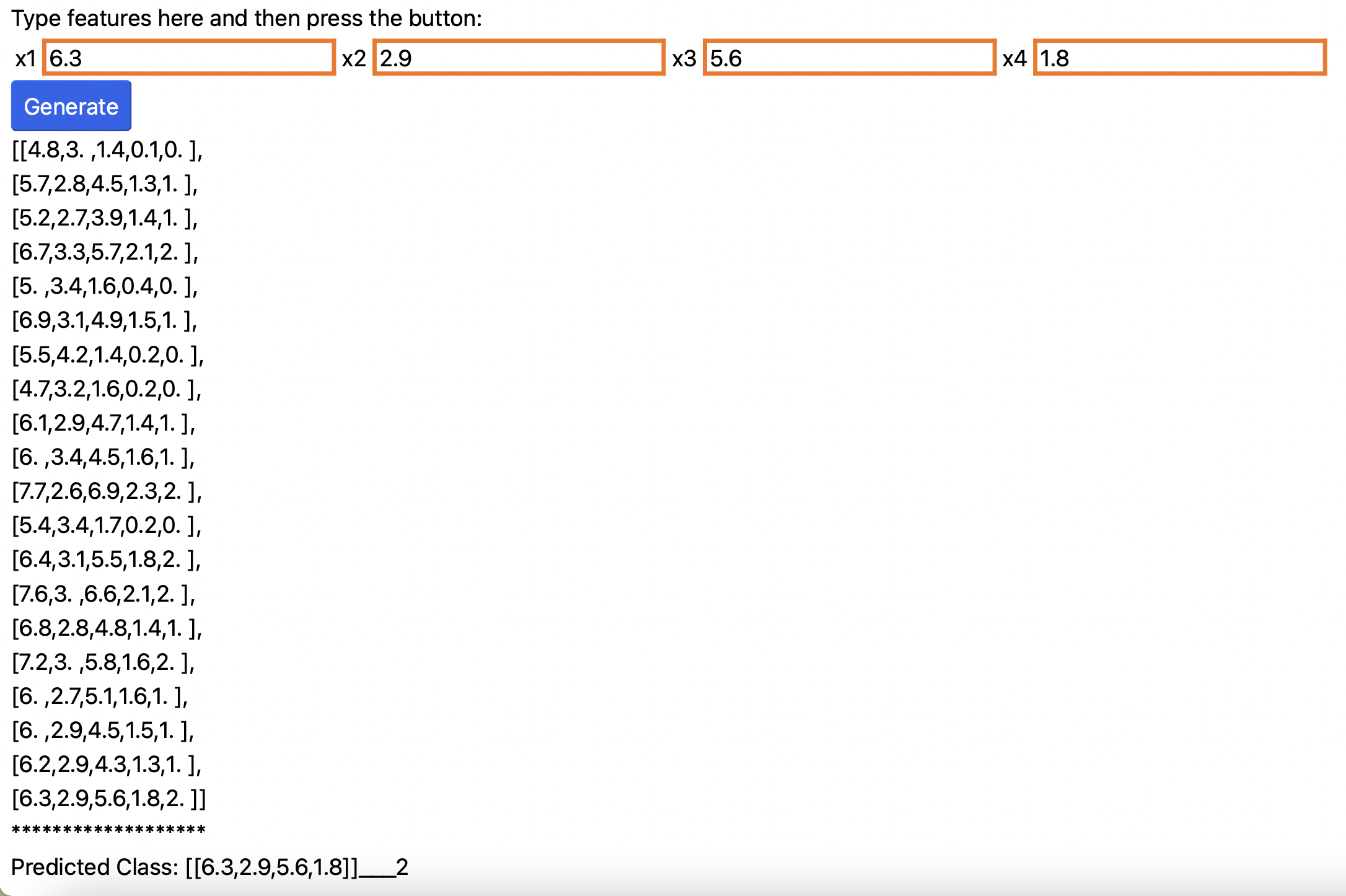
Well, that is it! The next figure shows what the final website should look like. For your convenience I have displayed in the website all the
test samples with their associated classes. If you notice, each row is a vector of 5 values separated by comma. The first four values are the 4
features (\textbf{[x1, x2, x3, x4]}), and the fifth value is the label. You can use this to make sure your model is predicting correctly.
Since it should not have seen the test samples before, it is possible that the model could make a few mistakes. However, if it is a good model,
for the majority of the cases, the predicted class should match the real class. With this idea, could you devise a metric to quantify performance?
You can call it the accuracy metric.
Note: you will get a few mis-classifications. But out of 30, it should be less that 5.
As an example, I grabbed the last test sample. I entered the 4 features into the text boxes, and the KNN model predicted the class 2.
If you look at the last data row in the figure, you can see that the label is also 2. Therefore, the model was accurate for that test sample.
Conclusion
This concludes this chapter. You have completed all the tasks and built and deployed your KNN website which can do Iris Flower classification. If you have not already realized it, you can build KNN models for other datasets or for your own data and problems. I hope this Volume 1 in the series sparks your imagination. I can't wait to hear what new applications you develop from the concepts in this book.