Chapter 3 - Traditional Machine Learning (Sample)

Copyright and License

Copyright © by Ricardo A. Calix.
All rights reserved. No part of this work may be reproduced or transmitted in any form or by any means, without written permission of the copyright owner.
MIT License.

FTC and Amazon Disclaimer

This post/page/article includes Amazon Affiliate links to products. This site receives income if you purchase through these links. This income helps support content such as this one.

Traditional Machine Learning

In this chapter, I will address some of the traditional machine learning topics. I will use python, numpy, and the Sklearn library to provide example code on how to use the different models and other tools. I will quickly move through KNN to arrive at other algorithms. Much of what we learn from using the SKlearn tool kit can be integrated with PyTorch to make your deep learning code more powerful and modular. That way, you will be able to re-use your code for many different tasks. I will not focus on the theory of traditional machine learning algorithms here. There are many books on the theory of machine learning algorithms so instead I will concentrate on the practical aspects of using them in Python. Machine Learning (ML) is essential to enable automated systems to make decisions and to infer new knowledge about the world. This section describes some of the most important traditional methodologies currently in use in the field of machine learning. Machine learning approaches can be divided into supervised learning (such as Support Vector Machines) and unsupervised learning (such as K-means clustering). Within supervised approaches, the learning methodologies can be divided, based on whether they predict a class or a magnitude, into classification and regression approaches, respectively. An additional categorization for ML methods depends on whether they use sequential or non-sequential data. Classifiers are machine learning approaches that produce as an output a specific class given some input features. Important classifiers include Support Vector Machines (Burges 1998) commonly implemented using LibSVM (Chang and Lin, 2001), Naïve Bayes, artificial neural networks, deep learning based neural networks, decision trees, random forests, and the k-nearest neighbor classifier. Regression models are those that produce a real valued number (magnitude) instead of a class such as the price or square footage of a house, or temperature, etc. Deep learning methods have made a big impact in the field of machine learning in recent years. In their simplest form, deep learning based methods are simply neural networks with more layers between inputs and outputs. In particular, they are very important because, given enough computational power, they can automatically learn the optimal features to be used in a ML model from the raw data. In the past, learning what features to use required using humans to engineer the features. This issue has now been alleviated considerably by deep learning. Additionally, artificial neural networks are models that can handle non-linearly separable data. In theory, this capability allows them to model data that may be more difficult to infer. DL methods have many more capabilities and some of them will be discussed in future chapters.

Code Issues

Before we begin, I want to address some issues about the code. First, I have tried to be consistent with other programmers of machine learning in Python. We will be using many libraries to implement the models. In particular, I selected to use the SKLearn library since it is very powerful and widely use. Especially for pre-processing steps. I only introduce enough SKlearn code for us to know how to integrate it with PyTorch in our deep learning endeavors. For a more in-depth discussion of SKlearn, I highly recommend the book “Python Machine Learning” by Sebastian Raschka. I have tried to be consistent with the conventions used in that book so that both books can be used together. So, now, getting back to the code, here is an example of some of the most important libraries that we can use for our machine learning modeling.

import numpy as np from sklearn import datasets from sklearn.cross_validation import train_test_split from sklearn.preprocessing import StandardScaler from sklearn.metrics import accuracy_score from matplotlib.colors import ListedColormap import matplotlib.pyplot as plt from sklearn.metrics import confusion_matrix from sklearn.metrics import precision_score from sklearn.metrics import recall_score, f1_score import pandas as pd from sklearn.preprocessing import LabelEncoder from sklearn import decomposition

As you may imagine, the SKlearn library is the main library which contains most of the traditional machine learning tools we will discuss in this chapter. The numpy library is essential for efficient matrix and linear algebra operations. For those with experience with MatLab, I can say that numpy is a way of performing linear algebra operations in Python similar to how they are done in MatLab. Using matrix and linear algebra operations makes the code more efficient in its implementation and faster as well. The datasets library seen above helps to obtain standard corpora (datasets). You can use it to obtain annotated data like Fisher’s iris data set, for instance. From sklearn.cross_validation} we can import train_test_split which is used to create splits in a data matrix such as using 70 \% for training purposes and 30 % for testing purposes. From sklearn.preprocessing we can import the StandardScaler module which helps to scale data. We can use functions such as these to scale our data for the PyTorch based models as well. Deep learning algorithms can improve significantly when data is properly scaled. So, it is recommended to do this. We will use the sklearn.metrics module for performance evaluation of the models. I will show that this module can be used with SKlearn models and with PyTorch models. Again, this will help to more easily understand deep learning since we do not have to use the more complex and very verbose PyTorch functions. The main metrics used to evaluate classification models are:

• accuracy_score
• recall_score
• f1_score
• precision_score
• confusion_matrix

The main metrics used to evaluate regression models are:

• coefficient of determination ($ R^2 $)
• RMSE

Two very important libraries are matplotlib.pyplot and Pandas. The matplotlib.pyplot library is very useful for visualization of data and results, and the Pandas library is very useful for pre-processing. The Pandas library can be very useful to pre-process large data sets in very fast and very efficient ways. There are some parameters that are sometimes useful to set in your code. The code sample below shows the use of np.set_printoptions, for instance. The function is used to print all values in a Numpy array. This can be useful when trying to visualize the contents of a large data set.

## set parameters np.set_printoptions(threshold=np.inf) ## print all values in numpy array

Now, let us assume that our data is stored in the matrix "X". The code segment below uses the function train_test_split}. This function is used to split a data set (in this case X) into 4 sets which are X_train, X_test, y_train, y_test. These are the 4 sets that will be used by the traditional or the deep learning models. The sets that start with "X" hold the input data (feature vectors) and the sets that start with "y" hold the output labels per sample. The values test_size=0.01 and random_state=42 in the function are parameters that define the split. The value 0.01 makes a train set that has 99 percent of all samples while the test set has 1 percent of all samples. In contrast, test_size=0.20 would mean that there is an 80 % and 20 % split. The random_state=42 allows you to always get the same random data since the seed is defined as 42.

X_train, X_test, y_train, y_test = train_test_split(X, y, test_size=0.30, random_state=48) ## k-folds cross validation all goes in train sets (hence 0.01) X_train, X_test, y_train, y_test = train_test_split(X, y, test_size=0.01, random_state=42)

To call all the functions or models you can employ the following approach. Here we have defined 5 common models. Notice that each one gets the 4 data sets obtained from the percentage split operation. Notice also that the data files have a _normalized added to their name. This is a good standard approach used by programmers to indicate that this data has been scaled (the next chapters address scaling). Here you run X_train through a scaler function to obtain X_train_normalized. The labels "y" are not scaled, in this case. Although they can be if needed.

logistic_regression_rc(X_train_normalized, y_train, X_test_normalized, y_test) svm_rc(X_train_normalized, y_train, X_test_normalized, y_test) random_forest_rc(X_train, y_train, X_test, y_test) knn_rc(X_train_normalized, y_train, X_test_normalized, y_test) multilayer_perceptron_rc(X_train_normalized, y_train, X_test_normalized, y_test)

Before we talk about the models, let us address Object Oriented Programming and performance evaluation. Performance evaluation will help you to determine how good your classifier (model) is, given an annotated test data set.

Object Oriented Programming

Object Oriented Programming (OOP) will be used extensively in this book to implement our ML and deep learning (DL) algorithms. As is necessary with progress, the DL algorithms are more complicated, with deeper and more resource intensive networks. This is best exemplified by one of the newest deep learning algorithms: The Transformer. The NN algorithms are just much more complicated. A little bit too much in fact and some proprietary programming libraries, as a result, are starting to abstract too much of the code. I have found that a simple solution to continue to write from scratch code is to write everything in an object oriented fashion. This way, you are still defining the classes from scratch but you can also build far more complicated algorithms thanks to traditional object oriented programming techniques. The following code segment includes a simple example of an OOP class format we will use extensively throughout this book for defining DL models.

class LinRegNet(nn.Module): ## init the class def __init__(self): super().__init__() self.linear1 = nn.Linear(11, 1) ## perform inference def forward(self, x): y_pred = self.linear1(x) return y_pred

In general, our OOP model classes will include an "init" function and "forward" function.

Performance Evaluation

As previously stated, performance evaluation depends on whether we are doing classification or regression.

Regression Performance Evaluation

The main metrics used to evaluate regression models are:

• Coefficient of determination ($ R^2 $)
• RMSE

My favorite regression evaluation metric is $ R^2 $. The range for the metric goes from 0-1 where 1 means that you have a good model. Generally, I have used sklearn \textbf{metrics} to evaluate regression models. If $ R^2 $ goes negative, then your model may not be learning the proper distribution. The code for $ R^2 $ can be seen in the following code listing:

## coefficient of determination (R**2) from sklearn.metrics import r2_score print( r2_score( y_pred.detach().numpy(), y_test.numpy() ) )

Classification Performance Evaluation

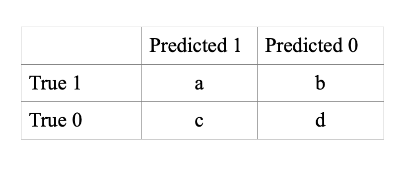
The main metrics to evaluate classification models are:

• accuracy score
• recall score
• f1 score
• precision score
• confusion matrix

Evaluation of the performance of your classifiers is extremely important. The SKlearn kit provides very good modules to address this issue. In particular, evaluation often involves measuring accuracy, precision, recall, and f-measure. The best way to understand these metrics is to think of a confusion matrix. Confusion matrices show how many elements from a class are correctly and incorrectly classified. For example, take the following:

Given this table, we can calculate accuracy as:

accuracy = (a+d) / (a + b + c + d)

Precision is defined as follows:

precision = a / (a + c)

The recall metric can be computed as follows:

recall = a / (a + b)

Finally, the "f" measure, which is a harmonic average of recall and precision, can be computed as follows:

F = (2 * (precision*recall)) / (precision + recall)

The sample code to obtain these metrics using sklearn is provided below.

from sklearn.metrics import confusion_matrix from sklearn.metrics import precision_score, recall_score, accuracy_score, f1_score def print_metrics_function(y_test, y_pred): print('Accuracy: %.2f' % accuracy_score(y_test, y_pred)) confmat = confusion_matrix(y_true=y_test, y_pred=y_pred) print("Confusion Matrix:") print(confmat) print('Precision: %.3f' % precision_score(y_true=y_test, y_pred=y_pred, average='weighted')) print('Recall: %.3f' % recall_score(y_true=y_test, y_pred=y_pred, average='weighted')) print('F1-measure: %.3f' % f1_score(y_true=y_test, y_pred=y_pred, average='weighted'))

The code above shows a function to print the performance metric statistics for a classifier. Notice that two sets are provided which are y_pred and y_test. The y_test data set contains the original annotated labels. The y_pred data set contains the labels predicted by your classifier. Each of the metric functions such as f1_score and recall_score uses these 2 data sets to calculate the respective metric. Generally speaking, the higher the better.

Plotting Performance

In the following code segment we can see the function plot_metric_per_epoch() which can be used to plot a metric value every N epochs. For this to work, you store the metric values in a list such as precision_scores_list and then proceed to plot these values using the "matplotlib" library.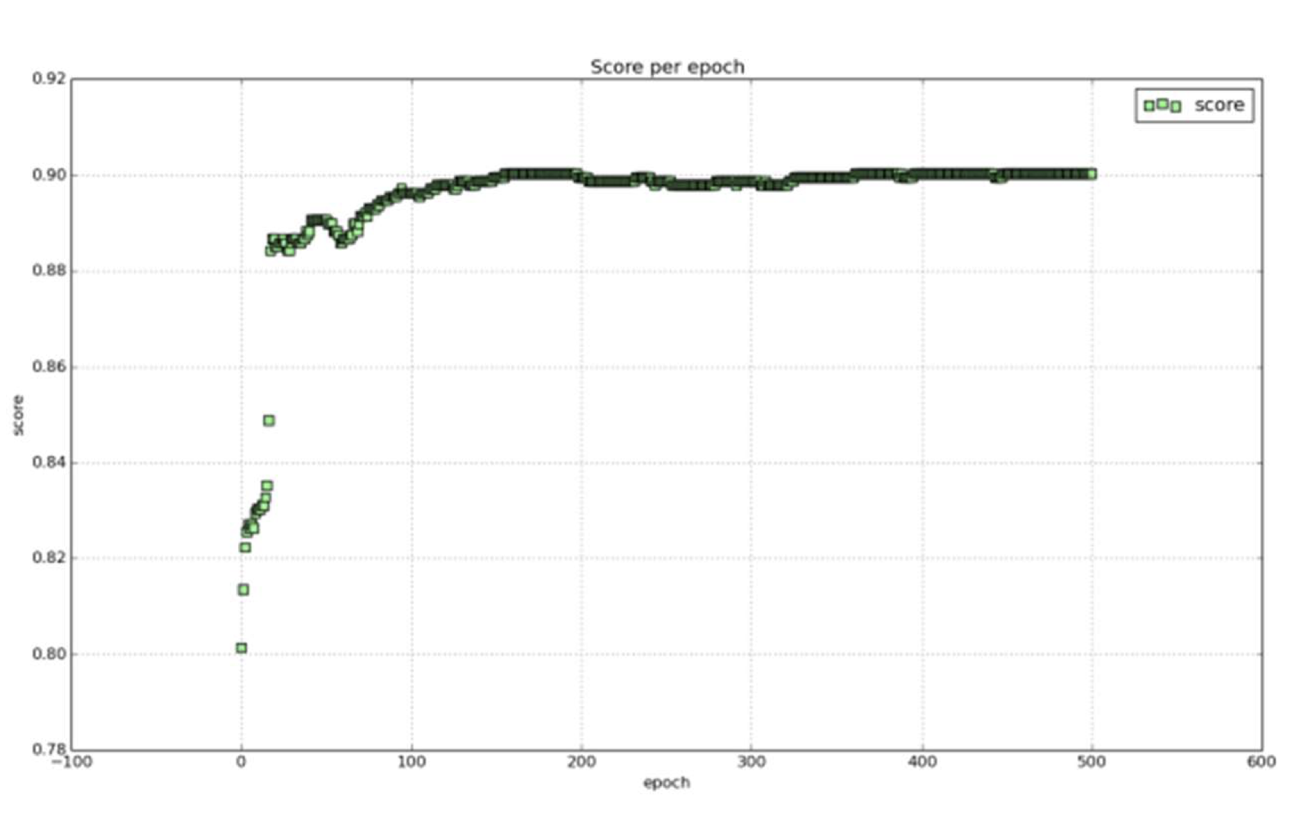

def plot_metric_per_epoch( precision_scores_list ): x_epochs = [] y_performance= [] for i, val in enumerate(precision_scores_list): x_epochs.append(i) y_performance.append(val) plt.scatter(x_epochs, y_performance,s=50,c='lightgreen', marker='s', label='score') plt.xlabel('epoch') plt.ylabel('score') plt.title('Score per epoch') plt.legend() plt.grid() plt.show()

The output should look like the following figure.

Information Theory

Information Theory provides a mathematical framework for quantifying information and uncertainty. Claude Shannon proposed metrics on how to measure the amount of information available (or not available) in a medium or that can be transmitted over a channel. These metrics include: Entropy, the Kullback–Leibler divergence, mutual information, among many others.

Entropy

Entropy is an idea in the context of information theory to describe uncertainty. For example, given a very biased coin with both sides having a tail, the probability of getting a head is 0 %. The chance of getting a tail is 100 %. So, we are 100 % sure of the outcome. Entropy, in this case, is 0 given that the uncertainty is 0. On the other hand, if we have a fair coin where both head and tail are equally likely; then, the uncertainty in this outcome is the highest. The formula for Entropy is as follows: \[ entropy = \sum -p \cdot ln(p ) \] You add or sum over all possible outcomes and "p" is the probability of each outcome. In the next graph, we plot the Entropy of a head for a fair coin given the probability of head.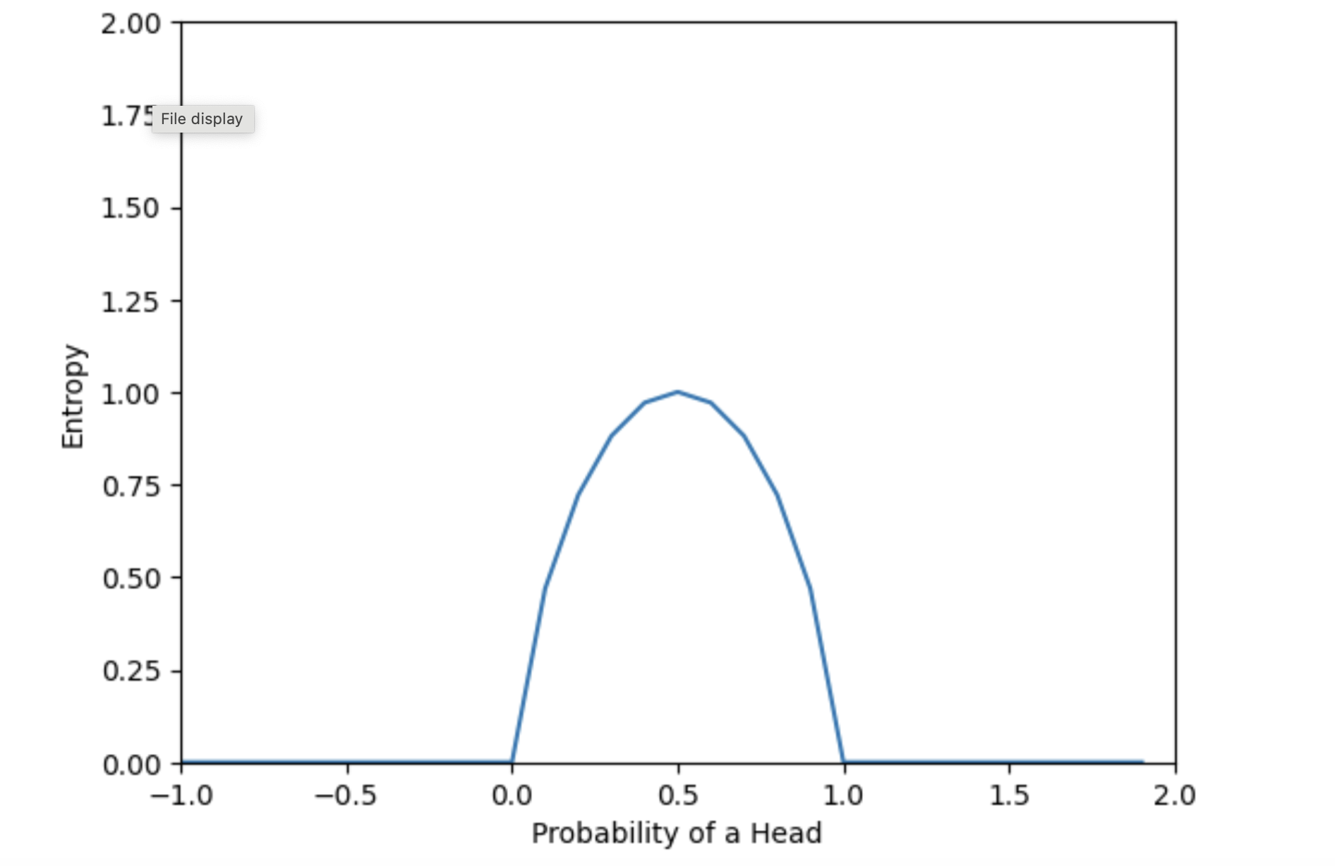

The top of the graph has the least certainty. At y = 0 (Entropy axis) you have the most certainty. When both sides of the coin are head (p(head)= 1.0), the uncertainty is equal to 0. When both sides of the coin are tail (p(tail)=1.0), the uncertainty is 0. The entropy (uncertainty) is highest when the coin is fair (p(head)=0.5). The code and data to generate the previous graph can be seen in the next code listing.

import matplotlib.pyplot as plt import numpy as np np.set_printoptions(suppress=True) def entropy_fn( p ): if p<=0 or p>=1: return 0 return -p * np.log2(p) - (1-p)*np.log2(1-p) xs = np.arange(-2,2,0.1) ys = [ entropy_fn(i) for i in xs ] print(xs) print(ys) plt.plot(xs, ys) plt.ylabel("Entropy") plt.xlabel("Probability of a Head") plt.xlim(-1, 2) plt.ylim(0, 2) plt.show() Result Data: [-2. -1.9 -1.8 -1.7 -1.6 -1.5 -1.4 -1.3 -1.2 -1.1 -1. -0.9 -0.8 -0.7 -0.6 -0.5 -0.4 -0.3 -0.2 -0.1 0. 0.1 0.2 0.3 0.4 0.5 0.6 0.7 0.8 0.9 1. 1.1 1.2 1.3 1.4 1.5 1.6 1.7 1.8 1.9] [0, 0, 0, 0, 0, 0, 0, 0, 0, 0, 0, 0, 0, 0, 0, 0, 0, 0, 0, 0, 8.960422633366421e-14, 0.4689955935892871, 0.7219280948873663, 0.8812908992306951, 0.9709505944546699, 1.0, 0.9709505944546672, 0.8812908992306896, 0.7219280948873574, 0.468995593589273, 0, 0, 0, 0, 0, 0, 0, 0, 0, 0]

Let us look at a couple of examples to better understand this concept. In example 1 we calculate entropy for a coin with both sides equal to head (unfair coin). Here we have: p(head)=1 and p(tail)=0. Entropy is calculated as follows: \[ entropy = \sum -p \cdot ln(p ) \] \[ entropy = -(1) \cdot ln(1 ) - (0) \cdot ln(0) \] \[ entropy = 0 \] In example 2 we calculate entropy of a fair coin so that p(Head)=0.5 and p(Tail)=0.5. This scenario should have the highest entropy and maximum uncertainty. \[ entropy = \sum -p \cdot ln(p ) \] \[ entropy = -(0.5) \cdot ln(0.5 ) - (0.5) \cdot ln(0.5) \] \[ entropy = 1.0 \] We can calculate this with python as well as can be seen in the next code listing.

def entropy_fn( p ): if p<=0 or p>=1: return 0 return -p * np.log2(p) - (1-p)*np.log2(1-p) p_ex2 = 0.5 Entropy_ex2 = entropy_fn( p_ex2 ) Entropy_ex2 ## 1.0

Kullback-Leibler (KL) divergence

The Kullback-Leibler (KL) divergence metric from information theory is designed to measure the difference between 2 distributions (P and Q). The formula for the Kullback-Leibler (KL) divergence is as follows:
$ D_{KL} ( p(x) || q(x) ) = \sum p(x) \cdot ln \frac{p(x)}{q(x)} $
A simple example of how to use the KL divergence can be seen in the next code listing.

import torch import torch.nn as nn import torch.nn.functional as F import matplotlib.pyplot as plt kl_loss = nn.KLDivLoss(reduction="batchmean") input = F.log_softmax( torch.randn(9, 8, requires_grad=True), dim=1) input.shape target = F.softmax(torch.rand(9, 8), dim=1) target.shape output = kl_loss(input, target) output ## tensor(0.4355, grad_fn=<DivBackward0>) ##################################### tensor2 = torch.rand(9, 8) * 3 + 2 tensor2 target2 = F.softmax(tensor2, dim=1) target2.shape output = kl_loss(input, target2) output ## tensor(0.7253, grad_fn=<DivBackward0>)

Notice here that "target2" is more divergent from "input" (0.72), than "target" is from "input" (0.43). PyTorch's KL divergence expects the input as log-probabilities (`log_softmax`) and the target as probabilities (`softmax`), the \(9\times8\) tensors represent a batch of 9 probability distributions with 8 values each rather than comparing only their means, and multiplying the second random tensor by 3 produces a generally more distinct probability distribution after applying softmax.

Mutual Information

Mutual Information (MI) is a metric that can be used to measure the relationship between one variable and another variable. In ML this can be used to measure the importance of features when predicting labels. For instance, we can use it to measure how much information we can get about one variable (labels) from another variable (features). We can see this with examples. In the next section I will contrast 2 cases (examples). I will create a data set that is 7x3 for "X", and 7x1 for "y". We will use MI to look at the importance of features when predicting the labels. In each of the 2 cases (example 1 and example 2), we will look at the MI between each feature and the labels. The higher the MI, the more related the features are to the labels.

from sklearn.feature_selection import mutual_info_classif import numpy as np ## f1,f2, f3, X = np.array([ [1, 1, 0], [1, 0, 1], [1, 1, 1], [0, 1, 0], [0, 0, 1], [0, 1, 0], [1, 0, 0] ] ) y = np.array( [0, 1, 1, 0, 1, 0, 0] ) mutual_info = mutual_info_classif(X, y, discrete_features=True) print("F1....", mutual_info[0] ) print("F2....", mutual_info[1] ) print("F3....", mutual_info[2] ) Results ## F1.... 0.014032215111297097 ## F2.... 0.0887819499348041 ## F3.... 0.6829081047004715

From the previous code listing, notice that the values of F3 are the most similar to the labels and as such have the highest MI. To better understand this concept, let us now intentionally increase the MI for F1. To do this we can make the values of F1 be more similar to the values of the labels. This makes the pattern more related and should increase the MI.

from sklearn.feature_selection import mutual_info_classif import numpy as np ## f1,f2, f3, X2 = np.array([ [1, 1, 0], [1, 0, 1], [1, 1, 1], [0, 1, 0], [1, 0, 1], [0, 1, 0], [0, 0, 0] ] ) y = np.array( [0, 1, 1, 0, 1, 0, 0] ) mutual_info = mutual_info_classif( X2, y, discrete_features=True ) print("F1....", mutual_info[0] ) print("F2....", mutual_info[1] ) print("F3....", mutual_info[2] ) Results: ## F1.... 0.36157373634686685 ## F2.... 0.0887819499348041 ## F3.... 0.6829081047004715

As can be seen, the MI of F1 has now gone up from 0.014 to 0.361.

Information Gain

Information Gain can be a useful metric in cyber security. It can help us to compare the entropy in 2 probability distributions. Let us consider a simple example. Assume you have 4 threats with associated probabilities. We are considering purchasing a new AI based security appliance. We have estimated the probabilities of the threat before and after purchasing the security appliance. We use Information Gain to begin to evaluate our outcomes. The example is presented in the following code listing:

from scipy.stats import entropy threat_before_new_appliance_probabilities = [0.2, 0.4, 0.3, 0.1 ] threat_after_new_appliance_probabilities = [0.2, 0.65, 0.1, 0.05] initial_entropy = entropy(threat_before_new_appliance_probabilities, base=2) after_entropy = entropy(threat_after_new_appliance_probabilities, base=2) information_gain = initial_entropy - after_entropy print("Initial Entropy (bits): ", initial_entropy ) print("Updated Entropy (bits): ", after_entropy ) print("Information Gain (bits): ", information_gain ) Result: Initial Entropy (bits): 1.8464393446710154 Updated Entropy (bits): 1.4166422780956525 Information Gain (bits): 0.429797066575363

From the results, we can see that the Appliance is good. There is an information gain (0.42) of using the appliance which means that there will be less surprise in the outcomes.

Conditional Entropy

Conditional Entropy (CE), like mutual information (MI), can be used to compare the relationship between variables (c and f). In fact, you can consider that MI(f, c) is related to entropy(c) minus CE(c|f). Conditional Entropy tells you how much surprise is left in "c" given that you know "f". This is best understood with 3 examples.

## High conditional uncertainty import numpy as np features = ["f1", "f1", "f1", "f1", "f1", "f1"] classes = ["c1", "c2", "c3", "c4", "c5", "c6"] joint_probs = {} for feature,the_class in zip( features, classes ): joint_probs[ (feature, the_class) ] = joint_probs.get((feature, the_class), 0) + 1 print( joint_probs ) joint_probs = {k: v / len(classes) for k, v in joint_probs.items()} print( joint_probs ) #################### marginal_probs = {} for feature in features: marginal_probs[feature] = marginal_probs.get(feature, 0) + 1 print( marginal_probs ) marginal_probs = {k: v / len(features) for k, v in marginal_probs.items()} print( marginal_probs ) ###################### conditional_entropy = 0 for (feature, the_class), p_joint in joint_probs.items(): conditional_entropy = conditional_entropy - p_joint * np.log2(p_joint / marginal_probs[feature]) print( conditional_entropy ) ## 2.584962500721156 ####################### outputs_probs = {} for item in classes: outputs_probs[item] = outputs_probs.get(item, 0) + 1 print( outputs_probs ) outputs_probs = {k: v / len( classes ) for k, v in outputs_probs.items()} print( outputs_probs ) outputs_only_entropy = -np.sum( [ p * np.log2(p) for k,p in outputs_probs.items() ] ) print( outputs_only_entropy ) ## 2.584962500721156

Notice that in example 1, we have 6 classes and all are equally conditioned by "f1". The variable f1 does not help to differentiate between the classes. So both the conditional entropy and the entropy of just the classes are the same. The "f1" does not help and as such you have a high conditional uncertainty. We know that the entropy of the class distribution alone is 2.58. And the conditional entropy is also 2.58. The "f1" is completely useless in this case.

## Medium conditional uncertainty features = ["f1", "f1", "f1", "f2", "f2", "f2"] classes = ["c1", "c2", "c3", "c4", "c5", "c6"] joint_probs = {} for feature,the_class in zip( features, classes ): joint_probs[ (feature, the_class) ] = joint_probs.get((feature, the_class), 0) + 1 print( joint_probs ) joint_probs = {k: v / len(classes) for k, v in joint_probs.items()} print( joint_probs ) marginal_probs = {} for feature in features: marginal_probs[feature] = marginal_probs.get(feature, 0) + 1 print( marginal_probs ) marginal_probs = {k: v / len(features) for k, v in marginal_probs.items()} print( marginal_probs ) conditional_entropy = 0 for (feature, the_class), p_joint in joint_probs.items(): conditional_entropy = conditional_entropy - p_joint * np.log2(p_joint / marginal_probs[feature]) print( conditional_entropy ) ## 1.5849625007211563 outputs_probs = {} for item in classes: outputs_probs[item] = outputs_probs.get(item, 0) + 1 print( outputs_probs ) outputs_probs = {k: v / len( classes ) for k, v in outputs_probs.items()} print( outputs_probs ) outputs_only_entropy = -np.sum( [ p * np.log2(p) for k,p in outputs_probs.items() ] ) print( outputs_only_entropy ) ## 2.584962500721156

The data for example 2 is now different. The first 3 classes depend on f1, and the last 3 classes depend on f2. Conditional entropy now tells you that knowing "f1" or "f2" helps, in general, to reduce the uncertainty of the class variable. We know that the entropy of the class distribution alone is 2.58. But, the conditional distribution is 1.58. Finally, in this next example we present the other extreme case.

## Low conditional uncertainty features = ["f1", "f2", "f3", "f4", "f5", "f6"] classes = ["c1", "c2", "c3", "c4", "c5", "c6"] joint_probs = {} for feature,the_class in zip( features, classes ): joint_probs[ (feature, the_class) ] = joint_probs.get((feature, the_class), 0) + 1 print( joint_probs ) joint_probs = {k: v / len(classes) for k, v in joint_probs.items()} print( joint_probs ) marginal_probs = {} for feature in features: marginal_probs[feature] = marginal_probs.get(feature, 0) + 1 print( marginal_probs ) marginal_probs = {k: v / len(features) for k, v in marginal_probs.items()} print( marginal_probs ) conditional_entropy = 0 for (feature, the_class), p_joint in joint_probs.items(): conditional_entropy = conditional_entropy - p_joint * np.log2(p_joint / marginal_probs[feature]) print( conditional_entropy ) ## 0.0 outputs_probs = {} for item in classes: outputs_probs[item] = outputs_probs.get(item, 0) + 1 print( outputs_probs ) outputs_probs = {k: v / len( classes ) for k, v in outputs_probs.items()} print( outputs_probs ) outputs_only_entropy = -np.sum( [ p * np.log2(p) for k,p in outputs_probs.items() ] ) print( outputs_only_entropy ) ## 2.584962500721156

In this last example, the data is different. Now each class (c1, c2, ..., c6) depends only on a single feature (f1, f2, ..., f6), respectively. Another way of putting it is that if I know that the feature is "f3", then I know that the class is "c3". If I know that the feature is "f5", then I know that the class is "c5", and so on. Based on this, knowing the feature means that there is no surprise in the resulting class and the conditional entropy is 0.

Optimization

Before we begin to discuss some of the machine learning algorithms, I should also say something about optimization. Optimization is a key process in machine learning. Basically, any supervised learning algorithm needs to learn a prediction equation given a set of annotated data. This prediction function usually has a set of parameters that must be learned. However, the question is “how do you learn these parameters?” The answer is that you do so through: Optimization. In its simplest form, optimization consists of trying many sets of parameters with your model and seeing what result they give you. If the result is not good, the optimization algorithm needs to decide if you should decrease the values of the parameters or increase the values of the parameters. In general, you do this in a loop (increasing and decreasing the parameter values) until you find an optimal set of parameters. But one of the questions to answer here as you are looping is: \textbf{do the values go up or down in this iteration?} Well, as it turns out, there are methodologies based on calculus that help you to make this decision. Let us try to picture this with a graph (below).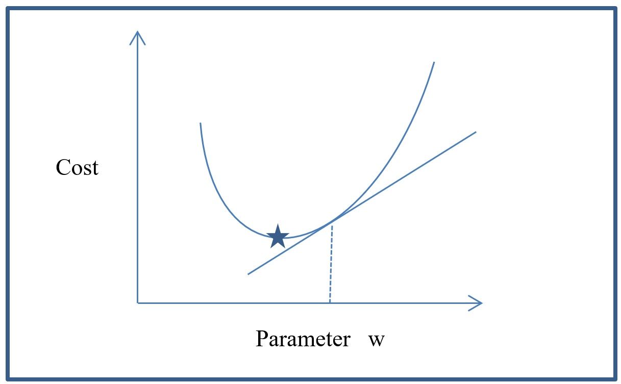

The above graph represents an optimization problem. The \textbf{y} axis represents the cost (or penalty) of using a given parameter. The \textbf{x} axis represents the value of the parameter (\textbf{w}) being used at the given iteration. The curve represents the behavior that the function (loss) being used to minimize the cost will follow for every value of parameter \textbf{w}. $ loss = ( \hat{y} - y )^2$ As shown in the graph, the optimal value for the curve is found where the star is located (i.e where the value of cost is at a minimum). So, somehow the optimization algorithm needs to travel through the function and arrive at the position indicated by the star. At that point, the value of \textbf{“w”} reduces the cost and finds the best solution. Instead of trying all values of \textbf{“w”} at random, the algorithm can make educated guesses about which direction to follow (up or down). To do this, we can use \textbf{calculus} to calculate the derivative of the function at a given point. This will allow us to determine the slope at that point. In the case of the graph, this represents the tangent line to the curve if we calculate the derivative at point \textbf{w}. If we calculate the slope at the position of the star symbol, then the slope is zero because the tangent at that point is parallel to the \textbf{x} axis. The slope at the point \textbf{“w”} will be positive. Based on this result, we can tell the direction we want to take for parameter \textbf{w} (decrease or increase). This type of optimization is called gradient descent and is very important in machine learning and deep learning. There are several approaches to implement gradient descent and this is just the simplest explanation for conceptual purposes. We can write the algorithm for this technique as follows:

old_x = 0 new_x = 4 step_size = 0.01 precision = 0.00001 def function_derivative(x): return 3*x ** 2 – 6*x while absolute_value(new_x – old_x) > precision: old_x= new_x new_x = old_x – step_size * function_derivative(old_x) print(“result is: ”, new_x)

In the previous code example we assume a loss function of: $ f() = x^3 - 3 x^2 + 7 $ that needs to be optimized for parameter \textbf{x}. We will need the value of the derivative for each point x. The derivative for f() is: $ f '() = 3 x^2 - 6x $ So, the parameter \textbf{x} can be calculated in a loop using the derivative function which will determine the direction to follow when increasing or decreasing the parameter \textbf{x}.

Anomaly Detection Algorithms

Perhaps the first set of machine learning algorithms to discuss in a "Cyber Security and Machine Learning" book is the set of algorithms related to Anomaly Detection. There are no machine learning algorithms exclusively for cyber security. Instead, there are many machine learning algorithms that can be applied to cyber security. Anomaly detection algorithms, as the name implies, seem to correlate well with cyber security problems. So what is special about an anomaly detection algorithm? Essentially, I would say that the key characteristic is that you do not need labels for the data samples. Usually in machine learning you have "X" and "y". Where "X" is the data of samples with features, and "y" includes the labels. Anomaly detection algorithms do not have associated labels. They are unsupervised. In this case, the machine learning model must learn what the data looks like. Once trained, the model can be used to compare new test samples to the learned distribution and determine if the test sample is similar or anomalous. There are several algorithms that can fit in this category. Some of them include: Hopfield networks (\cite{hopfield1982Ref}), Boltzman Machines (\cite{hinton1985Ref}), clustering, auto-encoders, etc. Clustering will be covered in the next sections in the context of KNN. Auto-encoders will be covered after deep learning is introduced in the next chapters. Throughout this book I will provide examples of how to use these for cyber security problems.

Hopfield Networks

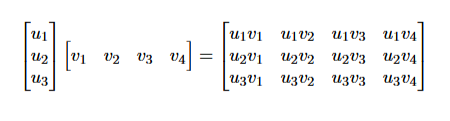
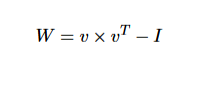
Hopfield Networks (\cite{hopfield1982Ref}) are sometimes called associative memory networks. John Hopfield won the 2024 nobel prize in physics for this work. They can be related to Information Theory because they can be used to store and re-construct (retrieve) information. The number of neurons can determine the amount of information that can be stored in the model. Hopfield Networks use the "outer product" multiplication to calculate the weights matrix. The "outer product" is an operation in linear algebra which, given 2 vectors, can return a matrix. The "outer product" operation can be seen in the next example: \[ \begin{bmatrix} u_1 \\ u_2 \\ u_3 \\ \end{bmatrix} \begin{bmatrix} v_1 & v_2 & v_3 & v_4 \\ \end{bmatrix} = \begin{bmatrix} u_1 v_1 & u_1 v_2 & u_1 v_3 & u_1 v_4 \\ u_2 v_1 & u_2 v_2 & u_2 v_3 & u_2 v_4 \\ u_3 v_1 & u_3 v_2 & u_3 v_3 & u_3 v_4 \\ \end{bmatrix} \] The weights are calculated via an "outer product" of the input vector and the transpose of the same vector. The identity matrix is subtracted from the resulting matrix as can be seen in the following formulation. \[ W = v \times v^T - I \] The weights are calculated using the "outer product" of the input vector and the transpose of the same vector. The outer product itself is simply $$ W' = vv^T $$ or, for each element, $$ w'_{ij} = v_i v_j. $$ In a Hopfield network, neurons are not connected to themselves. Therefore, the diagonal elements of the final weight matrix must be set to zero. For bipolar input vectors, where $$ v_i \in \{-1,1\} $$ the diagonal elements produced by the outer product are all equal to one since $$ v_i^2=1 $$ These self-connections can therefore be removed by subtracting the identity matrix: $$ W = vv^T - I $$ Equivalently, each individual Hopfield weight can be written as $$ w_{ij} = v_i v_j - \delta_{ij} $$ where \(\delta_{ij}\) is the Kronecker delta, defined as $$ \delta_{ij} = \begin{cases} 1, & i=j \\ 0, & i\neq j. \end{cases} $$ For example, consider the bipolar input vector $$ v = \begin{bmatrix} 1\\ -1\\ 1 \end{bmatrix}. $$ First, the outer product is calculated: $$ vv^T = \begin{bmatrix} 1\\ -1\\ 1 \end{bmatrix} \begin{bmatrix} 1 & -1 & 1 \end{bmatrix} = \begin{bmatrix} 1 & -1 & 1\\ -1 & 1 & -1\\ 1 & -1 & 1 \end{bmatrix}. $$ The Hopfield algorithm then removes the self-connections by subtracting the identity matrix: $$ W = vv^T-I = \begin{bmatrix} 1 & -1 & 1\\ -1 & 1 & -1\\ 1 & -1 & 1 \end{bmatrix} - \begin{bmatrix} 1 & 0 & 0\\ 0 & 1 & 0\\ 0 & 0 & 1 \end{bmatrix} = \begin{bmatrix} 0 & -1 & 1\\ -1 & 0 & -1\\ 1 & -1 & 0 \end{bmatrix}. $$ Notice that the outer product creates the initial matrix of pairwise relationships, while subtracting the identity matrix is a Hopfield-specific step used to eliminate the self-connections. Here are some important points to note about Hopfield networks and the code:

• np.outer produces one product between each possible element pairing from two vectors
• np.outer is used to calculate the "outer product"
• The outer product captures pairwise relationships between the features of a sample
• During training, these pairwise relationships are accumulated across the normal samples and stored in the weights matrix
• The Hopfield network can therefore be thought of as an associative memory of the normal patterns
• A new sample can be reconstructed using this stored memory and compared with its reconstructed version
• A large Hamming distance between the original and reconstructed samples may indicate an anomaly
• The Hebbian learning rule can be used for training

The following code segments provide an example of the basic idea with Hopfield networks for anomaly detection. First we define the Hopfield network and create some random data.

import torch import numpy as np class HopfieldNet: def __init__(self, size): self.size = size self.weights = np.zeros( (size, size) ) def train(self, patterns): for p in patterns: ## self.weights += np.outer(p, p) self.weights = self.weights + np.outer(p, p) np.fill_diagonal( self.weights, 0 ) # No self-connections ## self.weights /= len(patterns) self.weights = self.weights / len(patterns) def reconstruct(self, pattern, steps=10): for _ in range(steps): pattern = np.sign( np.dot( self.weights, pattern) ) return pattern data = np.array( [ [1, 1, 1, -1, 1, 1], # Sample 1 (normal) [1, 1, -1, 1, 1, 1], # Sample 2 (normal) [1, 1, 1, -1, 1, 1], # Sample 3 (normal) [1, 1, 1, -1, 1, 1], # Sample 4 (normal) ] ) hopfield = HopfieldNet( size=6 ) hopfield.weights hopfield.train( data )

After training, we can use the model to find anomalies. We take an input sample and reconstruct it through the network to create an output. We measure the hamming distance between input and output. A higher hamming distance may indicate anomaly.

def hamming_distance(a, b): """ Calculate the Hamming distance between two strings. """ ## arr1 = np.array(list(str1), dtype=int) # XOR to find differing bits, then count the number of 1s return np.count_nonzero(a != b) ######################################## ## normal sample test_sample = [1, 1, 1, -1, 1, 1] recalled_sample = hopfield.reconstruct(test_sample) print("Test sample: ", test_sample) print("Recalled sample: ", recalled_sample) test_sample_tr = torch.from_numpy( np.array( test_sample ) ) recalled_sample_tr = torch.from_numpy( recalled_sample ) distance = hamming_distance(test_sample_tr, recalled_sample_tr) print( distance ) ## Test sample: [1, 1, 1, -1, 1, 1] ## Recalled sample: [ 1. 1. 1. -1. 1. 1.] ## distance: 0 ###################################### ## abnormal sample test_sample = [-1, -1, 1, -1, -1, -1] recalled_sample = hopfield.reconstruct(test_sample) print("Test sample: ", test_sample) print("Recalled sample: ", recalled_sample) test_sample_tr = torch.from_numpy( np.array( test_sample ) ) recalled_sample_tr = torch.from_numpy( recalled_sample ) distance = hamming_distance(test_sample_tr, recalled_sample_tr) print( distance ) ## Test sample: [-1, -1, 1, -1, -1, -1] ## Recalled sample: [-1. -1. -1. 1. -1. -1.] ## Distance: 2

As can be seen in the previous code listing, the normal sample resulted in a hamming distance of 0. Whereas the abnormal sample resulted in a hamming distance of 2. Finally, Hopfield networks are considered a type of storage approach and have been called associative memory networks. As such, you can assign to them the information theory metric of "Storage Capacity". This metric helps to measure the limit in the number of samples the network can store. Storage capacity can be defined as follows: \[ Storage Capacity \simeq \frac{d}{2 log(d)} \] where "d" is the dimensionality of the sample vectors. The storage capacity of a Hopfield network depends on the number of neurons \(d\), which in this example corresponds to the dimensionality of the input samples. For example, a network with 1,000 neurons has an estimated storage capacity of approximately 72 representative patterns or memories. The network does not need to store every observed sample; instead, these stored patterns can represent characteristic states against which new samples can be recalled and compared.

import numpy as np d_vals = [6, 100, 1000, 10000] for d in d_vals: storage_capacity = d / (2 * np.log(d)) print("Neurons:", d, "Storage Capacity:", round(storage_capacity, 2))

The previous code produces approximately the following results:

• Neurons: 6 Storage Capacity: 1.67
• Neurons: 100 Storage Capacity: 10.86
• Neurons: 1000 Storage Capacity: 72.38
• Neurons: 10000 Storage Capacity: 542.87

It is important to note that storage capacity can be defined in different ways depending on the reliability requirements imposed on the Hopfield network. The approximation $$ C \simeq \frac{d}{2\ln(d)} $$ provides a conservative estimate associated with highly reliable storage and recall of random patterns. Another commonly cited result for classical Hopfield networks is approximately $$ C \simeq 0.138d $$ which uses a less restrictive criterion for successful recall. Therefore, storage capacity should be interpreted as an approximate measure that depends on how successful memory storage and retrieval are defined.

Boltzman Machines

Boltzman Machines (\cite{hinton1985Ref}) build on the idea of Hopfield networks and can be used to discover properties in data or anomalies. Geoffrey Hinton won the 2024 nobel prize in physics for this work. I will cover Restricted Boltzman Machines (RBMs) in this book, but not in this chapter. The reason for this is that RBMs are based on neural networks. Therefore, I will cover them in the network security chapter after I have introduced many concepts related to neural networks.

Popular Supervised Learning Algorithms

In this section, I will discuss some traditional and popular supervised learning algorithms. These are the ones that learn to correlate data to labels.

KNN

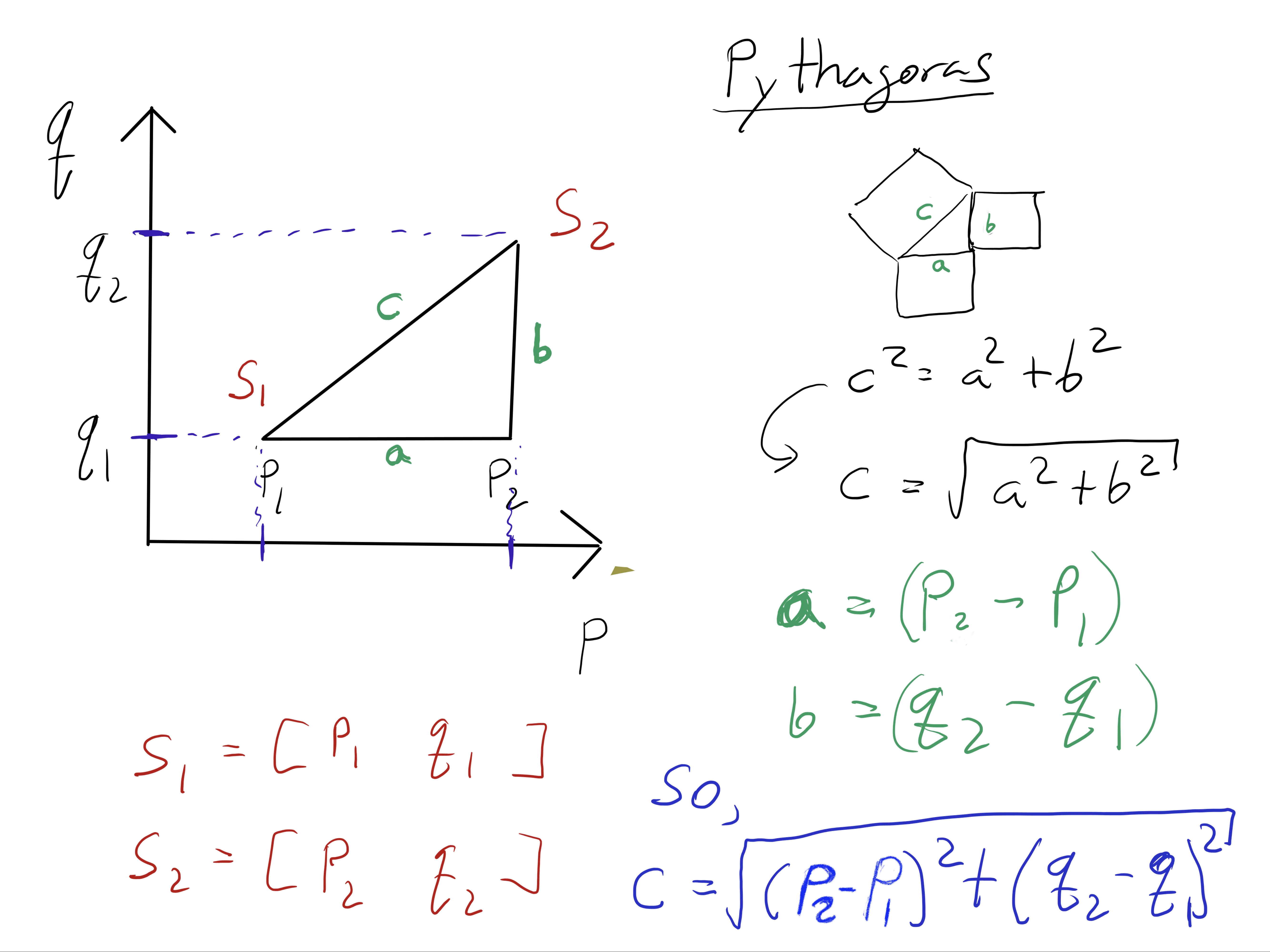
The k-nearest neighbor (KNN) classifier is a popular algorithm that I always like to use. It requires very little parameter tuning and can be easily implemented. Here, the KNN code is implemented in pure Numpy because of its simplicity. In this case, the \textbf{k} closest samples are selected. In the next code listings, you can see all the code needed to run KNN. Wow! Pretty short right? This code splits our data into \textbf{train} and \textbf{test} sets. Then grabs every sample in the test set and compares it to every sample in the train set. For each test sample, we get all distances between the test sample and all train samples. We then rank the distances and select the closest \textbf{K} distances. Finally, we assign the majority class associated with the closest 5 distances. That is it! Let us get started. First the libraries.

import numpy as np import pandas as pd import matplotlib.pyplot as plt import matplotlib.tri as tri from pyodide.http import open_url

Now we define the full KNN algorithm.

def euclidean_distance(v1, v2): return np.sqrt( np.sum( (v1 - v2)**2 ) ) def predict(test_x): k = 5 distances = [ euclidean_distance(test_x , x) for x in X_train ] k_neighbor_indices = np.argsort(distances)[:k] labels = [ y_train[i] for i in k_neighbor_indices ] labels_np = np.array( labels ) pred = int( np.mean(labels_np) ) return pred url1 = ("https://rcalix1.github.io/Build-Fun-AI-Projects-that-Run-on-the-Web/volume-1-pyscript-and-knn/chapter3/knn/iris.csv") iris_pd = pd.read_csv(open_url(url1)) iris_pd['species'] = iris_pd['species'].replace({'setosa':0, 'versicolor':1 , 'virginica':2}) iris_np = iris_pd.to_numpy() np.random.shuffle(iris_np) X_train = iris_np[1:130, :4] y_train = iris_np[1:130, 4] X_test = iris_np[130:150, :4] y_test = iris_np[130:150, 4] def my_gen_function(): accum_res = "" for i, test_x in enumerate( X_test ): the_pred = predict(test_x) my_gen_function()

The KNN code includes a function called the "Euclidean\_distance" as can be seen in the next code listing.

def euclidean_distance(v1, v2): return np.sqrt( np.sum( (v1 - v2)**2 ) )

This is the function that measures the distance between 2 points in a vector space. These 2 points need to have the same size but the size can be of any dimension. For instance, for the Iris data, every point has 4 features. So in the code the 2 points v1 and v2 would be of size 4 each. However, we could also have points (samples) of many more dimensions. For instance, points with 100 features. So in this case v1 and v2 would both need to have size 100. But the great thing is that the function for distance calculation would still work. That is the power of Numpy. The name Euclidean distance comes from a Greek philosopher named Euclid. He is best known for putting together one of the earliest books on geometry. The book was so good for its time that the type of mathematics it discussed became known as Euclidean geometry. So, where does this magical Euclidean distance function come from? Would you believe that it is related to an idea one of the great Greek philosophers (Pytagoras) is credited with? Pytagoras was before Euclid and is credited with coming up with the Pythagorean Theorem (bubble in the figure).

The theorem states that given a triangle (see figures), the sum of the areas of the two squares on the legs (a and b in green) equals the area of the square on the hypotenuse (c in green). If you look closely at the figure below, you can see that I have written down the connection between Pythagoras' theorem, and the Euclidean function we used in our code.

Now, with some of the math history out of the way, let us continue with our code description. In the next section we can see some of the details of the KNN \textbf{predict} function. Actually, the \textbf{predict} function is the actual KNN algorithm. I will describe it in detail next. The variable \textbf{test\_x} is the sample in question. Say, one Iris test sample with 4 features (\textbf{[x1, x2, x3, x4]}). The next line of code:

distances = [ euclidean\_distance(test\_x , x) for x in X\_train ]

calculates all the distances between \textbf{test_x} and all the training samples in \textbf{X_train}. The way this statement is written is called a list comprehension in Python. The \textbf{"for x"} part of the statement means that each sample in the train set is grabbed and passed to the \textbf{euclidean_distance} function along with the test sample. Both points are passed to the Euclidean equation and the distance between them is returned. This is done for every training sample and in the end, the list \textbf{"distances"} contains all the measured distances. The next statement:

k_neighbor_indices = np.argsort(distances)[:k]

takes all the distances and, using \textbf{np.argsort()}, sorts them. Then we slice the sorted vector with \textbf{[:k]}. This slicing only returns the indeces for the k smallest distances. The indeces are assigned to the array named \textbf{k\_neighbor\_indices}. One important note is that \textbf{"argsort"} returns only the indeces in the vector and not the values themselves. Since the indeces in the \textbf{"X"} data and \textbf{"y"} labels are aligned, then we can use these same indeces to extract the corresponding labels from \textbf{"y"}. And that is exactly what we do with the following statement:

labels = [ y_train[i] for i in k_neighbor_indices ]

Finally, the list \textbf{labels} is converted into a Numpy array of the labels which are numbers, and the mean of them is calculated. That is it. You have found the label. Wasn't that easy? We have described the whole KNN algorithm from scratch. Wow!

Logistic Regression

Logistic regression is a simple algorithm that is often used by practitioners of machine learning because it can obtain good results. Logistic regression is a linear function much like linear regression which predicts the probability of a sample belonging to a given class. Logistic regression uses another optimization function instead of the standard least squares cost function used in linear regression.

def logistic_regression_rc(X_train_normalized, y_train, X_test_normalized, y_test): from sklearn.linear_model import LogisticRegression lr = LogisticRegression(C=1000.0, random_state=0) lr.fit(X_train_normalized, y_train) y_pred = lr.predict(X_test_normalized) print_stats_percentage_train_test( "log re", y_test, y_pred)

The predicted values from a standard regression approach are now passed through a sigmoid function that basically maps the output to a probability range scale between 0 and 1. The code above provides an example of how to use the logistic regression function with SKlearn. Later, we will implement this logistic regression function again with PyTorch from scratch. In the previous function, the train and test sets are provided for the model to be trained and tested. In SKlearn most steps are abstracted. In contrast, PyTorch will allow us to define more steps such as the cost function, optimization, inference equation, and other aspects. In the function \textbf{logistic\_regression\_rc}, first you initialized a logistic regression object (lr) and then you train and test it with the functions \textbf{lr.fit} and \textbf{lr.predict}. The final step is to measure performance using the previously described function \textbf{print\_stats\_percentage\_train\_test}. Most classifiers are implemented in the same way with SKlearn. In the next section, I will demonstrate how this is done for a neural network in Sklearn.

Neural Networks

Neural networks can be very complex models that take a long time to train. Therefore, the use of them in SKlearn may not be recommended except for the smallest of data sets. The code is shown here for contrast purposes with later implementations of neural networks in PyTorch. In the next chapters, we will focus on how to do this in PyTorch and how to create networks of multiple layers from scratch. In the code below we can see that everything is very similar to the previous logistic regression implementation. The new changes appear in the definition of the \textbf{clf} multilayer object. Here, the parameter \textbf{hidden\_layer\_sizes}=(100,100) means that the architecture of the network consists of 2 hidden layers with 100 neurons each. A parameter such as (200, ) would mean that the network has 1 hidden layer with 200 neurons.

def multilayer_perceptron_rc(X_train_normalized, y_train, X_test_normalized, y_test): from sklearn.neural_network import MLPClassifier clf = MLPClassifier(solver='lbfgs', alpha=1e-5, hidden_layer_sizes=(100,100), random_state=1) clf.fit(X_train_normalized, y_train) y_pred = clf.predict(X_test_normalized) print_stats_percentage_train_test("multilayer perceptron", y_test, y_pred)

Regression, Trees, and XGBoost

There are several ML approaches to fit models to regression data. Three important ones are linear regression, regression trees, and neural networks. The next sections discuss regression and regression trees leading up to XGBoost. A more detailed discussion of regression will be covered later in the book.

Regression Trees

Regression trees (Torgo 2017) can fit nonlinear regression data. Regression trees are a type of decision tree in which the predicted values are not discrete classes but instead are real valued numbers. The key concept here is to use the features from the samples to build a tree. The nodes in the tree are decision points leading to leaves. The leaves contain values that are used to determine the final predicted regression value.

XGBoost

The "XGBoost" technique represents an improvement over other regression techniques like gradient boosting. XGBoost has new algorithms and approaches for generating the regression tree. It also has several optimizations that improve the speed and performance by which it can learn and process data. As of 2023, XGBoost can outperform many ML techniques including neural networks for small tabular data. XGBoost is also very easy to use and I would recommend always trying it with your tabular cyber security data. A usage example of XGBoost can be seen in the next code listing.

from xgboost import XGBRegressor from sklearn.datasets import load_boston from sklearn.datasets import fetch_california_housing housing = fetch_california_housing() boston = housing ## boston = load_boston() X = boston.data y = boston.target model = XGBRegressor() model.fit(X, y)

Summary

This chapter provided an overview of some of the main traditional topics in machine learning. In particular, the following machine learning algorithms were presented: anomaly detection, logistic regression, KNN, and neural networks. Code examples of their implementation using the sklearn toolkit or Numpy were presented and discussed. Additionally, issues related to classifier performance and information theory were also addressed. The next chapter will focus on issues related to data and data pre-processing that apply to "cyber security and machine learning".

Code Examples

• Example 1

Notes

Hopfield Networks

• Code Example: https://github.com/rcalix1/CyberSecurityAndMachineLearning/blob/main/FirstEdition/Ch3_TraditionalML/HopfieldNetworks.ipynb

Hopfield Networks

• We discussed the perceptron. Now it is time to connect multiple neurons together
• we now make the output of one neuron into the input to another neuron
• and this allows us to create neural networks
• Neural Nets can be of 2 types:
• a) Feedforward Nets (all in one direction - directed acyclic graph)
• b) Feedback nets (if not feedforward, then a network is a feed back net)
• This classification depends on their connectivity

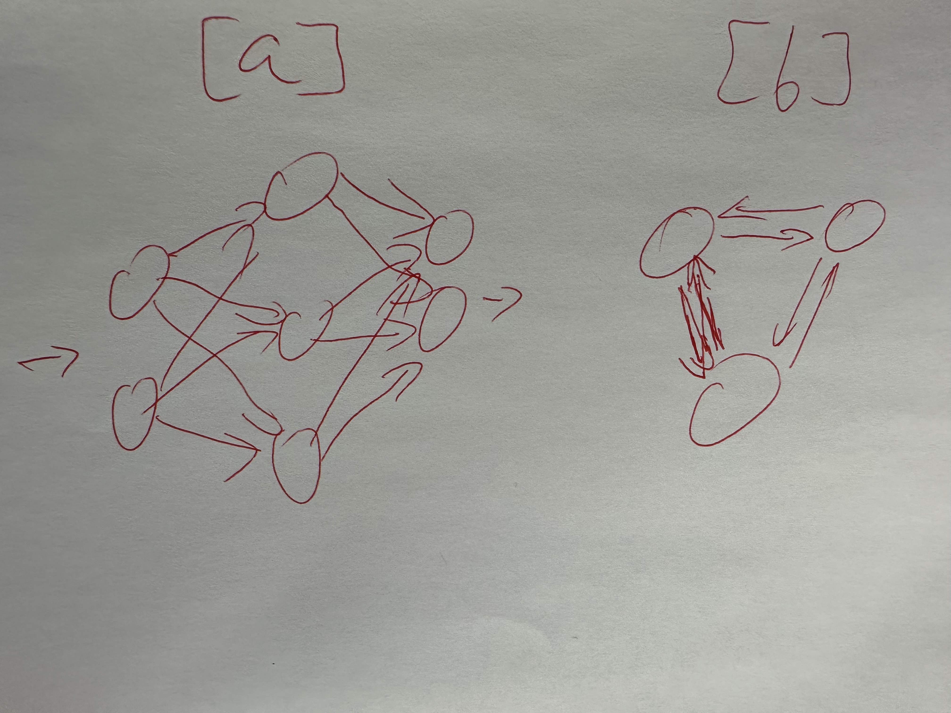
• they have been used to study associative memory. Memory can be used for anomaly detection, for instance

Hebbian Training

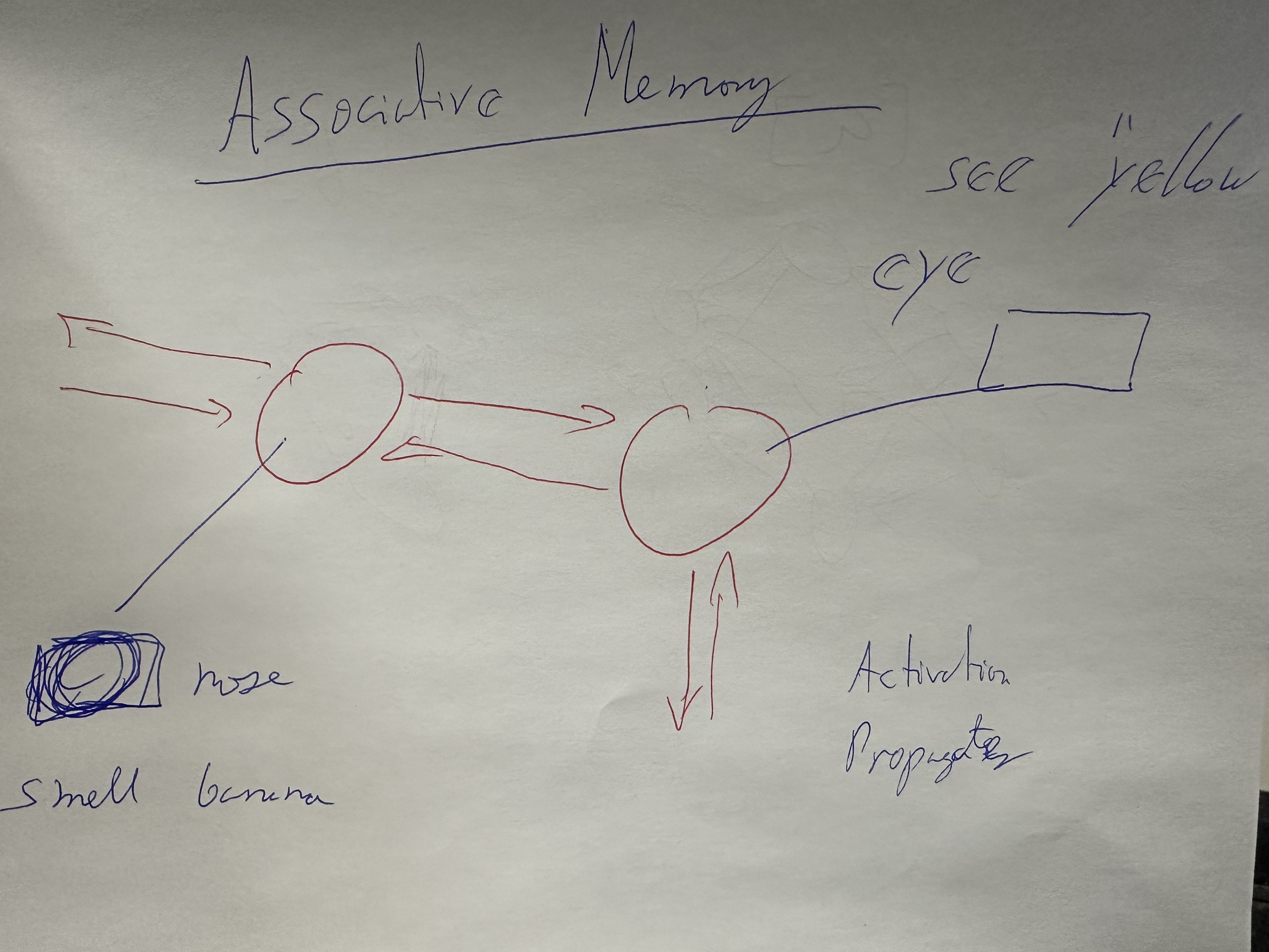
• Hopfield Networks are sometimes called associative memory networks.
• John Hopfield won the 2024 nobel prize in physics for this work.
• They can be related to Information Theory because they can be used to store and re-construct (retrieve) information.
• The number of neurons can determine the amount of information that can be stored in the model.
• Hopfield Networks use the "outer product" multiplication to calculate the weights matrix.
• The "outer product" is an operation in linear algebra which, given 2 vectors, can return a matrix.
• The "outer product" operation can be seen in the next example:

• The weights are calculated via an "outer product" of the input vector and the transpose of the same vector.
• The identity matrix is subtracted from the resulting matrix as can be seen in the following formulation.

Here are some important points to note about Hopfield networks and the code:

• np.outer produces one product between each possible element pairing from 2 tensors
• np.outer is used for the "outer product"
• The intuition is like a pairwise distance matrix
• This can help us to find the distance between each pair of point values