Chapter 4 - Data Loading and Pre-processing(Sample)
Copyright and License
Copyright © by Ricardo A. Calix.
All rights reserved. No part of this work may be reproduced or transmitted in any form or by any means, without written permission of the copyright owner.
MIT License.
FTC and Amazon Disclaimer
This post/page/article includes Amazon Affiliate links to products. This site receives income if you purchase through these links.
This income helps support content such as this one.
Data Loading and Pre-processing
In this chapter, I will address the very important issue of dealing with the data. To me and most practitioners, data processing is the most important issue
in machine learning.
There are many aspects that must be addressed when dealing with data. These include:
- getting the data
- cleaning the data
- pre-processing the data
- extracting the features
- building a corpus and annotating it
- performing inter-annotator agreement
- etc.
Here in this chapter I will address general issues about data as well as data issues related to cyber security and machine learning such
as one-hot encoding and feature extraction.
Loading the Data
Data can be obtained from the web such as text from twitter or web pages. Specific data sets can also be obtained from the machine learning libraries.
Sklearn has a “dataset” module, for instance. This dataset module can be used to obtain certain data sets such as the Iris dataset. An example of
this code can be seen below.
Here, the first index in the data matrix represents the rows and the second index represents the columns. Data can also be obtained from text files.
Many practitioners and academics will have their own data in text files. This data can be formatted in many different ways and loaded into the code.
In most of the examples in this book, the data is assumed to be formatted in csv (comma separated) format.
The code to load the data to both SKlearn based traditional machine learning algorithms and to PyTorch code files is shown below. In the code, we can see that
we can use the Numpy library (or namespace) to obtain the data. For the example below we assume that the data is stored in
the file \textbf{data/12559_Training_Dataset.csv} and is read by loadtxt() into the python variable \textbf{Matrix_data}.
Since we are using csv format, the Iris data file can look like the following.
Once the data is in \textbf{Matrix_data}, it can be processed as a Numpy array matrix. This means that it is no longer just an array but instead it
is more a vector or matrix as in linear algebra. Many operations are now simplified like extracting certain columns or rows. This is usually referred
to as slicing.
In the previous code listing we can see that we can calculate the dimensions of the matrix as follows:
And this gives you the number of columns or number of features plus the class.
Data and Feature Pre-Processing
Feature scaling is very important to achieving good results in ML modeling tasks. For example, in Principal Component Analysis (PCA) which is a feature reduction
technique, feature scaling is very important. The purpose of PCA is to project data to a space that captures the most variability in the data. If the features
are not scaled properly, one feature could dominate over the others and therefore be considered as the most variable feature.
With feature scaling, features with real valued numbers from any range can be mapped to other ranges such as from -1.0 to 1.0. This is performed for all features
so that no one feature will dominate in the model.
All machine learning models are susceptible to feature scaling. The code below shows how the data can be scaled from \textbf{X_train} to \textbf{X_train_normalized}.
CSV Files
In the following code listing I am showing you a general way in which you can take a standard dataset such as Iris or mnist obtained from a library module
and save it to a csv file.
This approach allows you to do the machine learning modeling by reading data from text files where the data is formatted in a very standard and well known
format such as csv (comma separated format).
One Hot Encoding
ML algorithm implementations in PyTorch use one-hot encoding. Quite simply, one hot encoding means that you take labels in the following format.
and convert them to labels in the equivalent one-hot encoded format as shown below. So, we create new vectors where all values are zero except for the
value of the position corresponding to the correct class in the vector.
One-hot encoding transforms the labels vector (\textbf{y}) of size \textbf{n} into a matrix of size \textbf{n} by \textbf{B} where \textbf{B} represents the number
of classes in the data set. For the case of the Iris dataset, we have 3 classes and, therefore, for a sample with label 2 we would get an equivalent one-hot
encoded vector equal to [0,0,1].
The code to convert the data to one-hot encoded format is provided below. There are several ways of implementing one-hot encoding. I have used the approach below
because I think it is the easiest to understand (while possibly not the most efficient or pythony).
Notice how \textbf{“a”} is a 2-dimensional array initialized with all zeros. You use the value in the input vector data to determine the
indeces \textbf{i} and \textbf{j} that are used to assign a "1" to the correct position in the matrix.
Features
A machine learning (ML) algorithm is only as good as the features that are provided to it. This statement used to be very true and many people made careers
of just developing features for problems in different domains. For instance, in NLP, many people would spend a lot of time developing parsers and other
techniques to find and create features from a text input. Similarly, in image processing, researchers developed many techniques to filter data out of images
to perform efficient image classification. Today, deep learning has somewhat changed this. DL has managed to introduce approaches to decrease the amount of
human involvement in the feature extraction process. Basically, deep learning (DL) methods, in some cases, have the ability to extract features from
raw data using only un-supervised or self-supervised techniques, transfer learning, etc. In some way, you can say that deep learning algorithms can extract
the features themselves without human involvement. This ability has had a very strong impact on the performance of the algorithms implemented in industry
and in the work performed by machine learning specialists. These abilities, for enhanced feature extraction, are available for the main ML mediums such as
for text processing and for image processing. I think they are less developed in the medium of Cyber Security.
In this section, I will cover ways of extracting features to address problems such as: malware detection, network intrusion detection, phishing detection, etc.
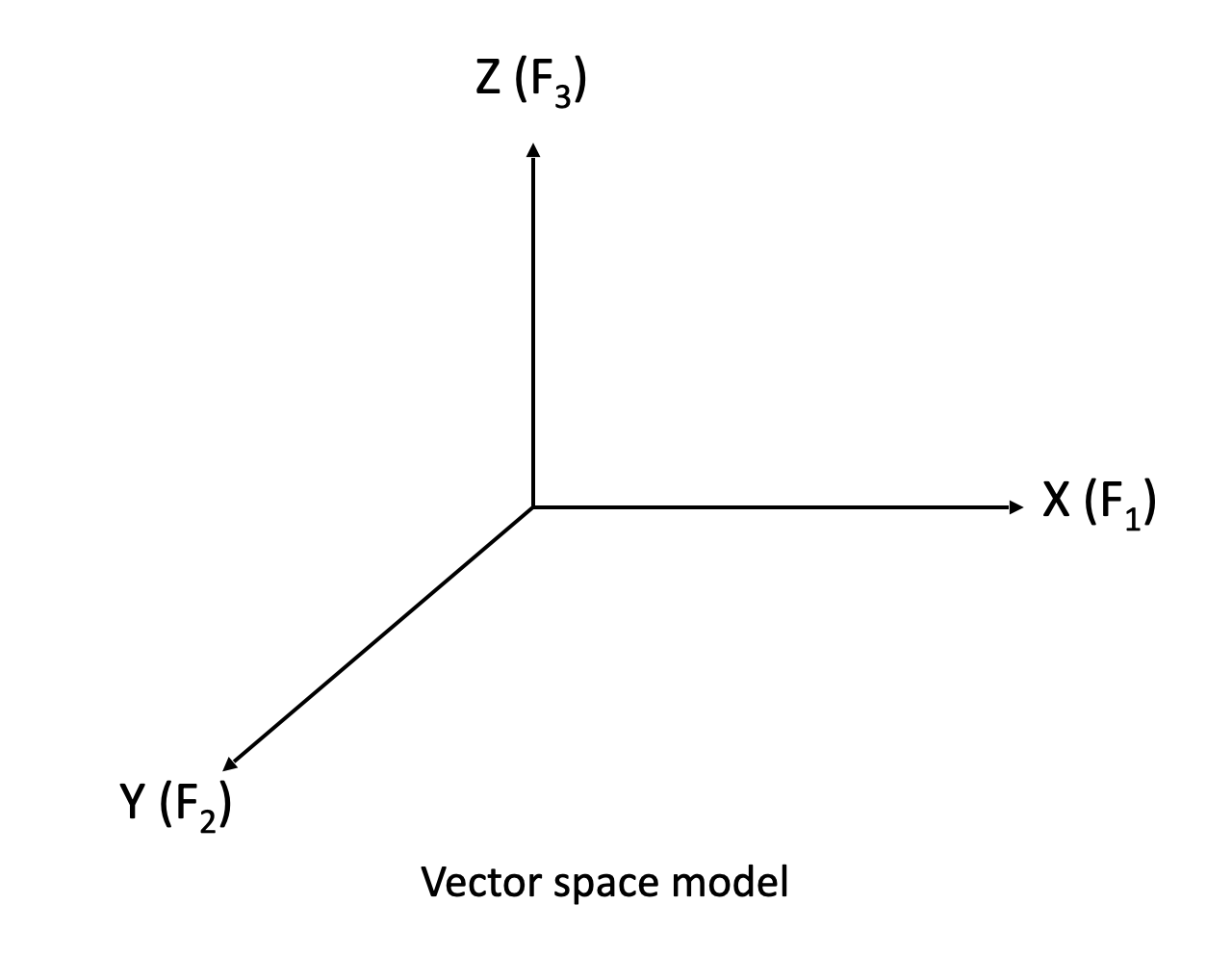
In general, we need techniques to extract data from cyber security related sources that we can convert to vector space model formats for use in machine
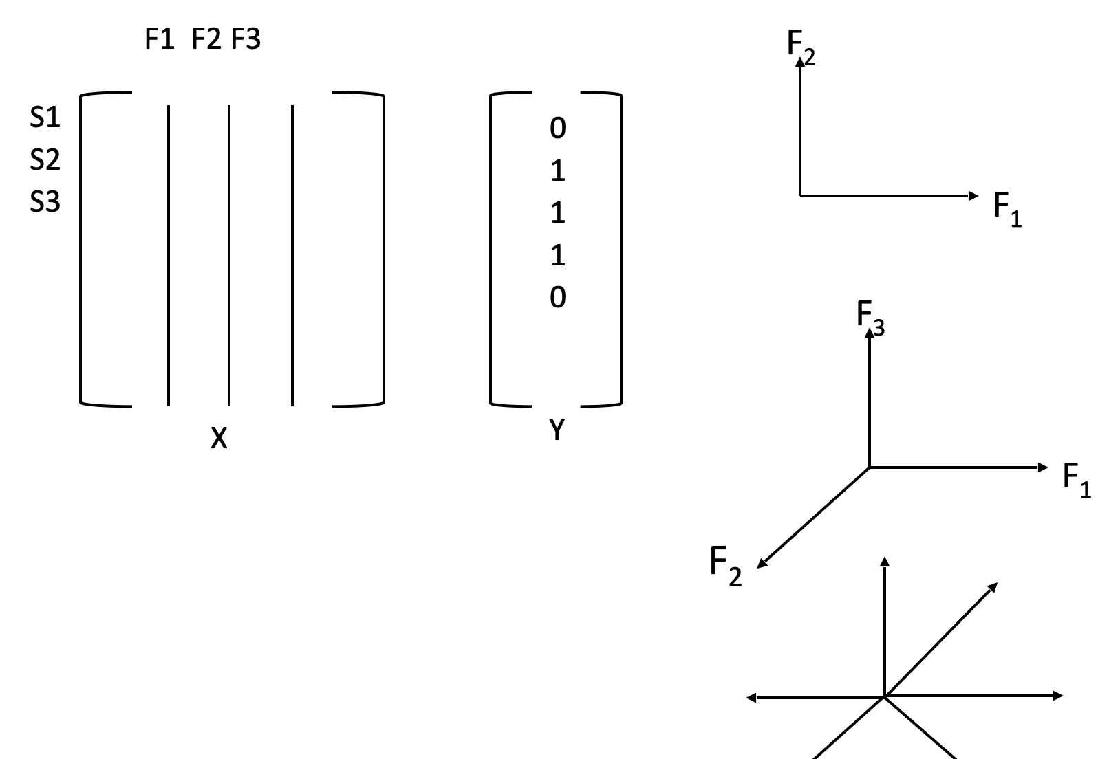
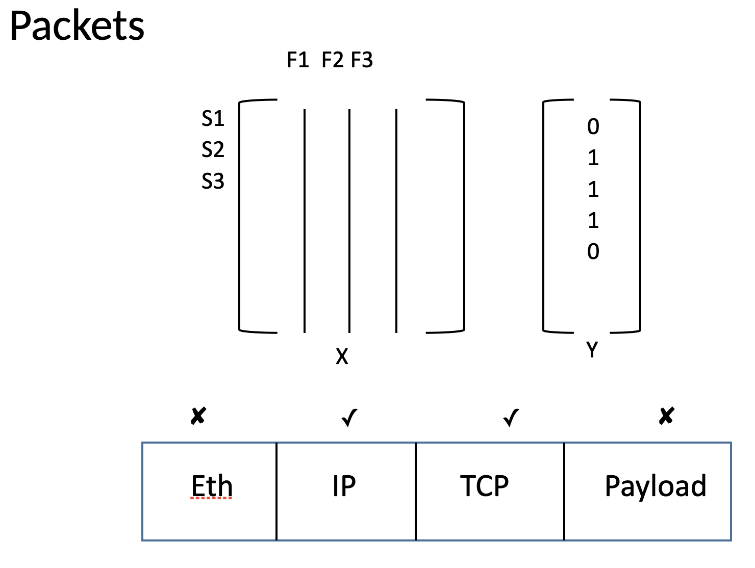
learning algorithms. The vector space model format is simply a comma separate file (CSV) where each column(F1, F2, F3, ...) maps to an axis in a vector
space (X, Y, Z, ...).
The columns are the axes on the vector space. An N number of columns corresponds to an N number of axes in the vector space ($R^N$).
Sniffing and Spoofing
When it comes to network data, sniffing and spoofing can be considered the two main approaches for network data processing and manipulation.
Sniffing can be more directly linked to defense and analysis, whereas spoofing can be more directly linked to attacks.
Sniffing
Sniffing is the process of capturing packets and extracting data from them. The following code listing shows an example of this using Scapy
(a Python library). You need to have root privileges on the computer to be able to sniff packets.
The code uses "sniff" with a filter to capture and print "icmp" packets.
Spoofing
Spoofing is the process of creating or modifying packets. Any packet that is arbitrarily modified by a user or agent can be used in an attack.
You need to have root privileges on the computer to be able to spoof packets.
The next code listing shows an example of how to spoof packets. Here we generate and send 10 ping packets to the address 8.8.8.8.
In the next code listing we can further modify the ping packets to carry a text message. Consider that here we have a delivery mechanism and think
of the text message as an actual payload that could be malicious.
The possibilities with Scapy are endless. For instance, here we can create a very simple script to simulate the "traceroute" functionality.
Features from Network Data
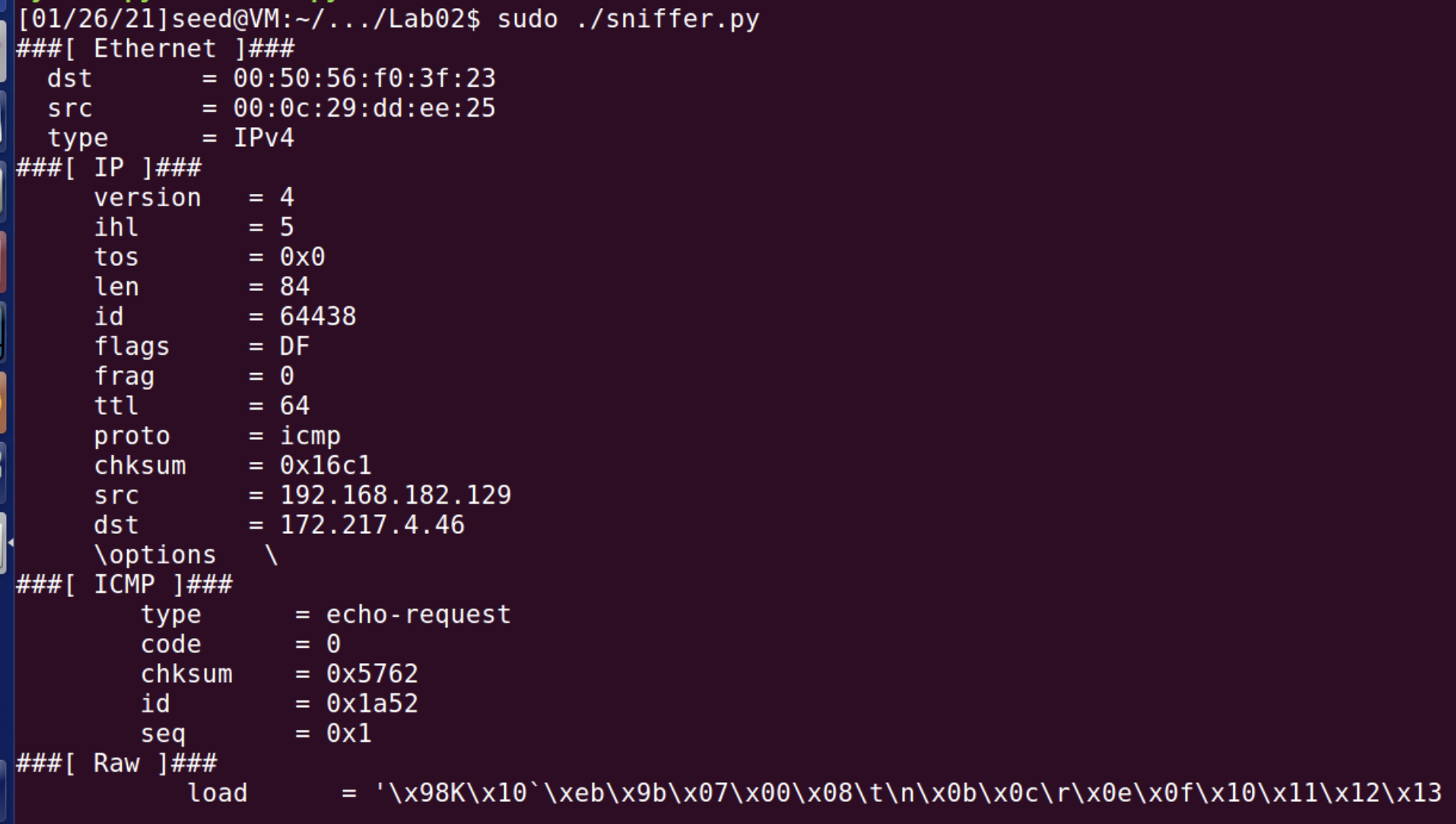
Sniffing is the process of collecting data from network packets. The Python Scapy library is great for this. In the next code listing
we see an example of how to collect network packet data from ping (icmp) packets using Scapy. The function "sniff" has a filter option to specify
what kinds of packets to collect (e.g. icmp, http, sport=80, etc.).
The results of running the sniffer can be seen in the following figure.
Example to extract features from PCAP files
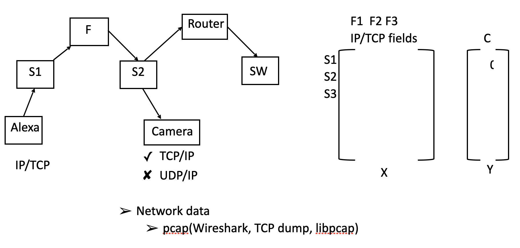
A PCAP file is a type of file used to store collected network data. For this example, for instance, we collected data from an IOT
(Internet Of Things) network environment. The goal is to go from data in the network (in the form of packets) to a vector space
representation of the data samples for use in ML applications. The following figure summarizes the pipeline.
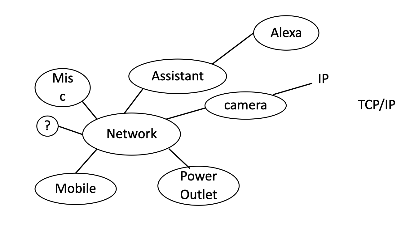
The IOT network consists of IP enabled devices such as cameras, assistants, etc. (next Figure).
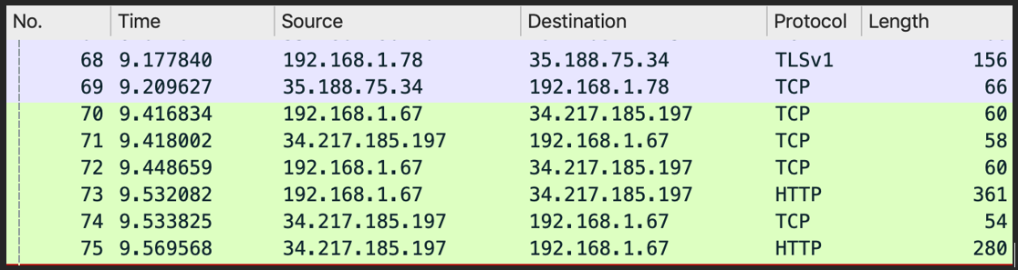
Sniffers such as Wireshark produce PCAP files (figure below).
In this example, we extract features from PCAP files in order to represent the raw data as feature vectors.
The PCAP file includes many columns. Here is a description of a few of the columns:
- No: The number of the packet in the captured file
- Time: The timestamp of the packet
- Source: The address where this packet is coming from
- Destination: The address where this packet is going to
- Protocol: The protocol name in a short (perhaps abbreviated) version
- Length: The length of each packet
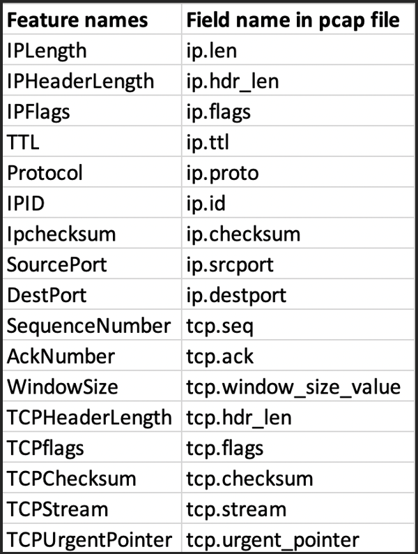
The following figure shows an example of some of the features we can use.
Every packet is made up of headers such as IP, TCP, etc. And each header can contain multiple fields (e.g. srcport, protocol, etc.).
The following code can be used to extract features from PCAP files. The PCAP files used in this example are available on the GitHub. First we filter
the PCAP file and then we extract features using "tshark". The results are written to a text file.
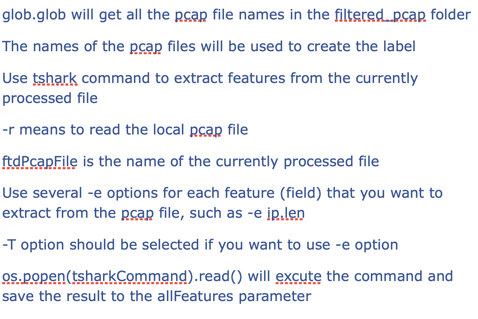
The "tshark" command includes several flags.
Some of the "tshark" flags from the previous code segment are described in the following figure.
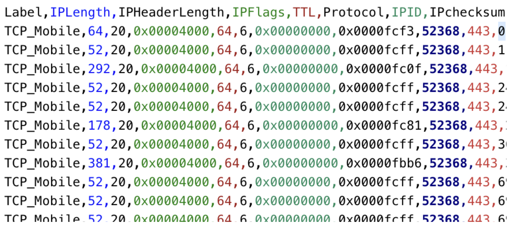
After running the previous code, the extracted features, written to the final text file, should look like the following.
As such, the fields in the packets are represented as columns in the CSV file (Next figure). The columns in the CSV will be used to extract "X" and "y" for
use in training the ML algorithms.
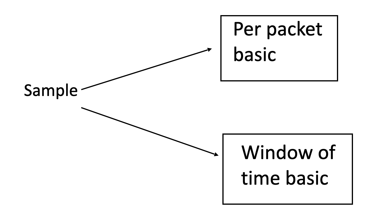
In the previous example, we defined each sample as being a single packet. However, that is not necessarily the only option. For instance, for detecting
denial of service attacks, we may need to use samples that include multiple packet information. In this case, instead of individual packets as samples,
we may need to create samples that include averages of multiple packet data given a window of time.
Features from Malware
Extracting features from malware can seem like a daunting task. But, in fact, this can be simple depending on the approach. In static malware analysis,
we do not need to run the malware in a sandbox environment and instead just extract data from the actual static malware files. This can be as simple
as the following:
Notice that in the previous code segment, we copy the "exe" file data into a bytearray. The function
extract_features()
is simpler than it seems. The "malwareByteArr" variable is now a sequence of data much like a string in Byte format. Common sequences of characters
can be extracted in a similar way to how you would process syllables in text.
We could, for instance, use a tokenizer as in the next code listing.
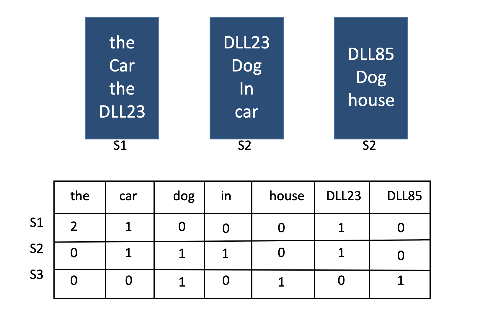
From here, we could use the "bag of words" approach to generate the CSV for use with ML algorithms. See \textbf{Bag of Words} approach in the next section.
This example will be covered in more detail in the Malware chapter.
Another type of malware analysis approach is called "Dynamic Malware Analysis". In dynamic malware analysis, we would generate a \textbf{log file} containing
information about the behavior of the malware after running it in a sandbox environment with an emulator.
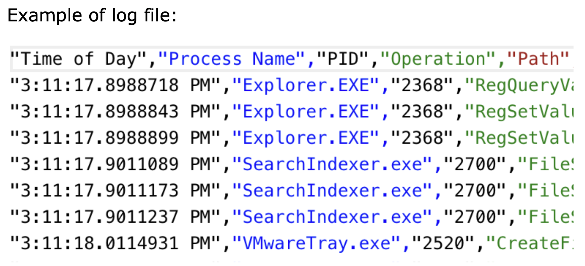
The following figure shows an example of a log file with malware behavior data (from dynamic analysis). The information in this file can include: file
read traces, DLL calls, registry edits, etc. DLL is the acronym for dynamic linked library. These are files that contain code, data, etc. that can
be used by several programs when running on the operating system.
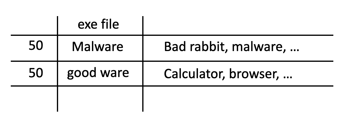
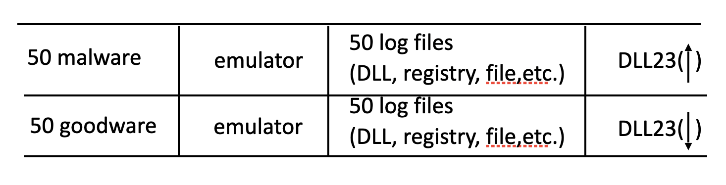
Let us consider a scenario where we have "exe" files (goodware and malware).
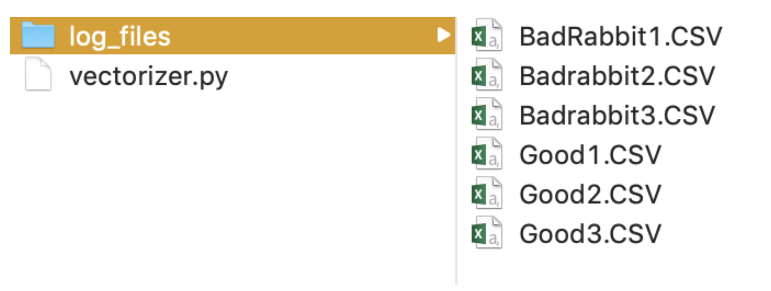
After running these "exe" files in an emulator, we could end up with a \textbf{log file} (CSV) for every goodware or malware sample (Figure below).
Each of these log files could become a sample in our \textbf{X} matrix for use in ML modeling. The contents of the log files could be the source to extract
the features for each sample.
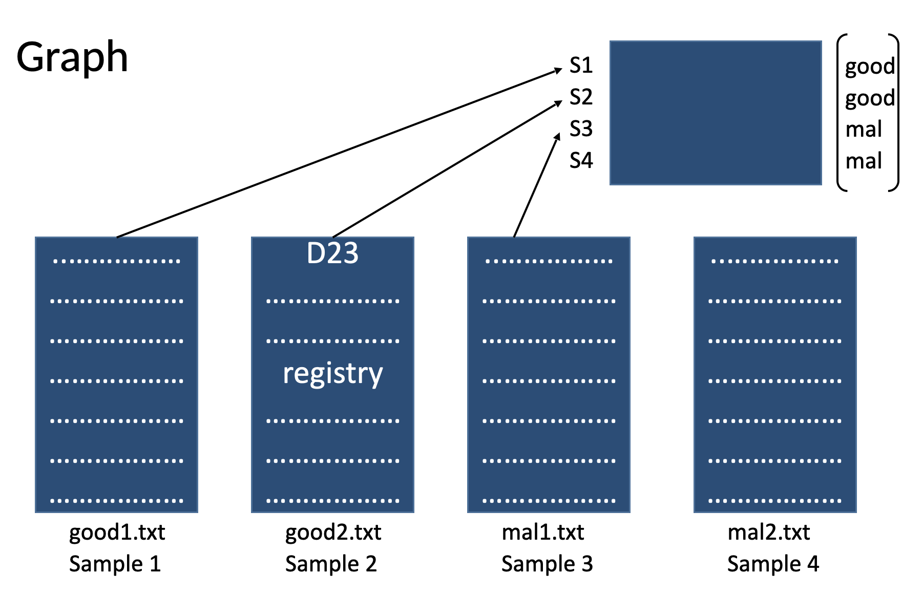
As can be seen in the next figure, each log file (s1, s2, etc.) is used to create the \textbf{X} matrix.
We can then combine the goodware and malware log files to create our data set with samples and labels.
For instance, we could have 50 samples of malware and 50 samples of goodware. This data is available on the GitHub and this example will be
covered further in the "Malware" chapter.
Each sample (S1, S2, ...) should be consistently represented by the same features such as DLL calls, registry edits, file read traces, etc.
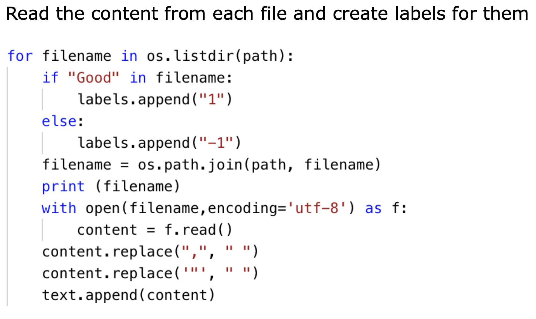
When we are extracting the features from the log files we can also add the labels using the file names (i.e. goodeware or malware). The code for this can be seen
in the next figure.
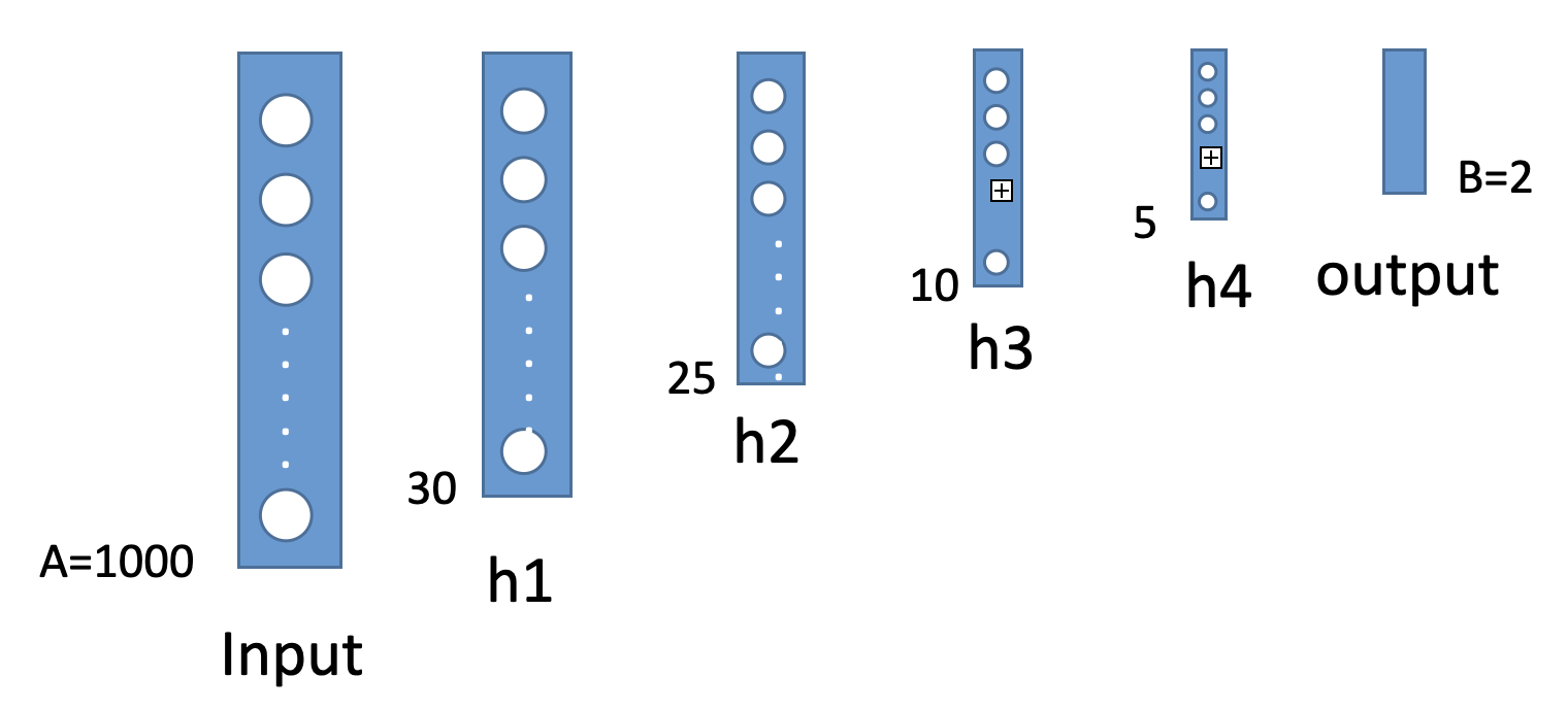
Once the data is extracted, we can proceed to build the neural network model (such as the following). This will be addressed further in the "Malware" chapter.
Features from Forensics
Digital forensics is a huge field and there are many techniques that fall under the topic. In this section I will show a simple example of how to extract
meta-data from an image file. Digital meta data has been used by law enforcement to solve many crimes.
The following code listing shows the example code. You can use any JPG file with this code.
The extracted forensic data should look like the following.
As can be seen, we have information about the OS, the software version, etc.
Features from Text
Feature extraction from text usually involves the processing of text documents to extract tokens, words, chunks, or other phrases to be used to create
the features. There are many, many types of features that can be extracted from text. Some of the methods (\babelEN{\cite{Jurafsky2008Ref}}) that can
be used include:
- the bag of words approach
- frequency histograms of the words
- Part of speech tagging of the words
-
- Anaphora resolution
- word embeddings (the main method used today)
With the information provided by the previous methods, many features can be extracted. In general, text features can be binary or numeric.
Binary features include the presence or absence of words, part of speech tags, chunks, syntactic parses, semantic parses, etc. Numeric
based text features can be derived from performing counts or calculating distance metrics between words or higher level semantic concepts such as with embeddings.
One simple technique, for example, that has had success in extracting features for supervised machine learning is called the gramulator
(McCarthy et al. 2012). The gramulator is a feature extraction technique used particularly in natural language processing.
The main idea is that, for a 2 class problem, you want to extract features (e.g. words or tokens) that are very frequent in one class but
infrequent in the other. This helps to better discriminate between the classes. The downside of this approach, however, is that it needs
a lot of annotated or labeled data to extract the grams or words from each class that are infrequent in the opposite class. If the grams
are representative of the entire population; then, it can be expected that a classifier will have good performance in the classification task.
The downside of most of these techniques is that in the past they have required annotated data. Deep learning provides several new techniques
that address this issue and obtain good performance without needing large amounts of annotated data. These mainly involve some type of word
embedding approach with self-learning. Word embeddings are vector representations of words or syllables or subwords. The vectors are dense
and usually of fixed size such as 256. The values of each vector representing the token in question are learned through some algorithmic
scheme such as Word2Vec (Mikolov et al. 2014), or Transformers.
These techniques can be very useful for cyber security.
Bag of Words approach
A very simple example of performing the "bag of words" approach can be seen in the next code listing. The code uses the "CountVectorizer" function
from sklearn to perform this task. We will use "CountVectorizer" with a concrete example in a future chapter.
Features from Websites for Web Security
Web security can relate to defending against web attacks such as SQL injections and cross site scripting attacks (XSS).
Web Attacks
- cross site scripting attacks (XSS)
- SQL injections
- cross site request forgery
The following code listing shows how to extract features for use in addressing these types of attacks. In particular we can use the
python "beautifulsoup" library to extract data from HTML files.
Here, the approach in the code looks for occurrences of the "script" tag, for instance.
Features from Images
Feature extraction from images is another area where deep learning is revolutionizing the way features are engineered and obtained.
The input to a model when performing image processing and classification is an image. In general, images are 2 dimensional arrays that
contain the pixel intensities that define the image. For color images, you have 3 two-dimensional matrices where each stores the
intensity for the R, G, and B color channels of the image.
Traditional Image Feature Extraction Techniques
In the past, these images where converted into feature vectors for use in machine learning using image processing based feature extraction techniques.
Again, here, researchers spent considerable amounts of time performing feature engineering. Some of the methods widely used in image
processing (\babelEN{\cite{Gonzales2007Ref}}) include:
- Image segmentation
- Edge detection
- Region growing
- Image morphing
- Fourier transformations
Many features could be extracted using these methods. Generally speaking, many of these techniques are implemented as a filter that
is applied to the images to convert them into another matrix of the same size or of another size. This new image will store new information about the
image such as the pixel positions where an edge was detected. Here, once again, deep learning changed how this process is done.
Deep neural networks can be used to discover the features simply by providing the raw inputs and some annotation (e.g. labels). This information alone allows
the neural network architecture to connect the neurons in ways where it can discover features by itself. In fact, deep neural networks are not just used for
classification anymore but can also be used just for feature extraction. ResNet is an example of this. The extracted features can then be used with other
classifiers such as SVM, logistic regression, etc. In these cases, the input layer and hidden layers are used for feature extraction without having to use the
output layer from the original classification task. Instead, the classification task can be changed to another task. Convolutional Neural Networks (CNNs)
can provide this functionality for image processing and classification.
A Class to Load Images into Tensors
Loading images into tensors can be challenging. The following code listing presents an object oriented approach to load images from files into PyTorch tensors.
This OOP class was written by my students Danielle Turner, David Higley, and Joseph Shapiro and I thank them for it.
First we import the libraries.
Next we define the class to load the images from folders into tensors.
The Dataset of images is in \textbf{data\_path} which is the path to the images folder. This should contain multiple folders of each class.
The current working directory is where the "pt" file will be stored. The "train" parameter is for whether to load train or test data.
The "transform" parameter indicates the Torch transform to apply to the image data. The "target_transform" is the transform to
apply to the targets if needed. The "convert" parameter is used to indicate if the data should be converted from images, or loaded from
a "pt" file. The "size" parameter is to set the size of the images to convert to. This should be the same as the size of the images
in the "pt" file (e.g. 226).
The next code segment includes the definitions of the "convert" and "load_functions" for the images.
The "convert" function in this OOP class is what converts the images to a defined size and then "center" crops them.
Corpora (i.e. Annotated Datasets)
A supervised machine learning algorithm is only as good as the data that is provided to it. ML models learn how human annotators assign the labels
to a sample and a system can only be expected to be as good as the human annotator. Some tasks are more subjective than others for human annotators and this
is usually reflected in the classifier performance. Therefore, many practitioners recommend, before measuring classifier performance, that an analysis of the
subjectivity of the human annotation should be performed. This is usually referred to as Inter Annotator Agreement.
When annotating (labeling) a new resource, the quality of the annotation process must be measured in some way. Inter-annotator metrics refer to techniques used to
measure the overall agreement between the annotations of two or more individuals (humans). Important metrics used to evaluate inter-annotator
agreement (\babelEN{\cite{artsteinRef}}) include:
- Average observed agreement
- Pi
- Alpha
- S
- Kappa
In general, these metrics differ in how they correct for expected chance agreement.
Expected chance agreement
Expected chance agreement is the probability that 2 annotators will agree on their annotation for an item by chance. This probability depends
on the number of classes. Formally, this probability is calculated as follows:
$ A_e = \sum_{k \in K} P( k | c_1) \cdot P(k | c_2) $
where $ c_i $ is the annotator $ i $ , and $ k $ is the assigned category. Inter-annotator agreement metrics are important because they help to set
theoretical boundaries on the accuracy that a given machine learning methodology can achieve using the annotated corpora (\babelEN{\cite{birdRef}}).
A brief description of some of the techniques is provided in the following discussion.
Average Observed Agreement (Ao)
Averaged observed agreement is the easiest metric to compute. It is the percentage of annotations that two annotators agreed upon. The metric is
formulated as follows where the variable \textbf{“samples”} represents the total number of annotation samples, and \textbf{“agreed”} is the amount
of samples for which both annotators agreed.
$ A_o = \frac{1}{samples} \sum Agreed $
Chance-corrected Metrics (Acorr)
Chance corrected metrics are those that take into account the \textbf{expected} chance agreement \textbf{Ae}. Once chance agreement is defined,
the metric can be corrected. These types of metrics include: \textbf{s}, \textbf{alpha}, and \textbf{kappa}. Formally, the main concept in these
metrics is defined as follows:
$ A_{corr} = \frac{A_o - A_e}{1 - A_e} $
The following code segment shows how to perform this analysis using the well known \textbf{nltk} framework ( www.nltk.org ).
More details about data collection, corpora development, and web scraping can be found from the following sources: Web Scraping with Python by
Ryan Mitchell, Calix and Knapp (2011), and Natural Language Processing with Python by Bird, Klein, and Loper.
Summary
In this chapter, a discussion about issues related to data and data pre-processing was provided. In particular, the following topics were addressed:
data pre-processing, reading data from csv files, types of features, corpora processing, and one-hot encoding. In the next chapter, we will
begin our discussion of how to program out first deep learning models with PyTorch.