Chapter 10 - Transformers

Transformers are the latest step in the evolution of deep learning. As is necessary with progress, newer deep learning algorithms are also much more complicated, with deeper and more resource intensive networks. The Transformer is the best example of this. Transformers are, for me, the first algorithm I was not able to run on a laptop when using a significantly large data set. They truly require a machine learning “war machine”. Lots of GPU power and memory, etc. The algorithms are much more complicated, as you will see, and the networks are very deep. Transformers are one of the new innovations in NLP since 2017. They were first made popular by the paper “Attention Is All You Need” by (Vaswani et al.). They are very interesting and seem to be very powerful. Currently, they are better than Recurrent Neural Networks (RNNs) for NLP because they parallelize better and because of the Attention mechanism. So far, Transformers have been used to develop very impressive implementations such as BERT (Devlin et al. 2018), and GPT-3 (Radford et al. 2019), and most notably, chatGPT from OpenAI, as of this writing. ChatGPT in particular seems to be very good at language understanding. Transformers have also been applied to language translation, question answering, document summarization, automatic code generation, text generation, etc. In general, something like chatGPT requires at least 2 steps. One step is called the Pre-Training process and the other step is called fine tuning. Basically, a Transformer network is trained on all the data you have (e.g. all text data in the world). This process requires massive amounts of computing and can be very expensive. The most notable pre-trained GPTs include: GPT-3, GPT-4, and LlaMa models, to name a few. The next step is to fine tune the model. Once the fine tuning is complete, you have options such as adding more neural net layers after the transformer and freezing the already pre-trained weights. Or you can just keep training the transformer for a specific task and have all the weights be changed. The amount of fine tuning data does not need to be as large as the data for pre-training. In fact, it can be orders of magnitude smaller. Okay, let’s get started.

Copyright and License

Copyright © by Ricardo A. Calix.
All rights reserved. No part of this work may be reproduced or transmitted in any form or by any means, without written permission of the copyright owner.
MIT License.

FTC and Amazon Disclaimer

This post/page/article includes Amazon Affiliate links to products. This site receives income if you purchase through these links. This income helps support content such as this one.

Main Ideas of the Transformer

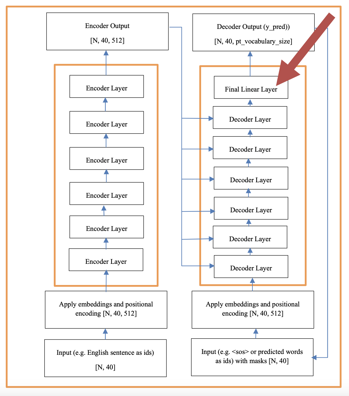
So, where does one start with Transformers? The Transformer is complex and it involves several ideas to make it work correctly. In this section I will present the main ideas first with some relevant code. Understanding these concepts or steps really well before venturing to write the code for the Transformers is really important. It will save you time in the long run. So now, let us proceed to discuss these topics. In the next sections I will start discussing the code for GPTs, BERTs, the full Encoder Decoder transformer architecture, and a few other subjects. As can be seen in the previous figure, the original Transformer consisted of an Encoder and a Decoder layer.

Numpy arrays, tensors, and linear algebra

Linear algebra, numpy arrays, and tensor operations are at the heart of understanding the Transformer architecture. Before you continue, I strongly recommend that you read and practice the topics in chapter 1, and in particular, the section on linear algebra, numpy arrays, and tensor operations.

Attention

The Attention mechanism in Transformers is the heart of the whole algorithm. The attention matrix is nothing more than a dot product matrix multiplication between all the tokens (e.g. words, syllables, subwords, etc.) in a sentence (e.g. the input English sentence). The idea is that, given the input and output, the model learns to correlate the words in the sentence to determine their importance. This is done multiple times and that is why it is called a multi head attention mechanism.

Embeddings

Sequences of tokens in a sentence are converted into sequences of IDs. An Embedding approach converts the sequence of ids into a sequence of embeddings. You will go from a 2d tensor

[N_batches, _tokens]
to a 3d tensor of size:
[N_batches, N_tokens , embedding_dimension ]
The term N_tokens can also be called seq_length_max. Here N_batches is the batch size, N_tokens or seq_length_max is 40, and embedding_dimension is 512. The term N_tokens (i.e. 40) just establishes the size of the input sentences we wiil allow. Sentences in Transformers are not of variable length. Instead you define a buffer size to hold the sentence. If the sentence is too long, then it is truncated. If the sentence is too short, then the buffer is padded. The embedding size is selected arbitrarily like in word2vec.

Masks

Masks serve several purposes. One is to help ignore the padded values during training. The other goal is to block the given word you want to predict or future words). This brings up the important aspect of training with Transformers. Transformers predict the last word in a sequence. For example:

Given an input in english: "the cat is sleeping"

a Transformer is also given part of the output sentence. In this case: "el gato esta ?". The Transformer will predict the next word in the sequence which in this case would be "durmiendo" to complete the translation as “el gato esta durmiendo”. All of this is achieved through the masks to ignore padded values and to only show the partial sentence.

Positional Encoding

This is the technique that allows you to encode sequence. Transformers are all about being parallel. Their direct competitor is Recurrent Neural Networks (RNNs). RNNs have had several problems in the past. One is that they do not scale well to GPUs and parallel approaches because of their recurrence and dependence on previous steps. The other problem is the famous "vanishing gradients" problem which was addressed by by residuals and LSTMs seem to have addressed this now. Transformers did away with the type of sequence modeling approach used in RNNs all together so they are very good for parallel approaches. But how do they address or encode the sequence? Obviously knowing that the word "cat" goes before the word "sleeping" is useful. This is where a technique called positional encoding comes into play. Basically, after embedding, you have a vector per token of, say, size 512. Now, with positional encoding, a function that calculates sines and cosines, is used to create a new vector also of size 512 that represents position (i.e. sequence) of the tokens. The 2 vectors are added together (embedding + positional_encoding) to get the new inputs to the network. Also, the position vector values are smaller than the embedding vector values so as to not let position dominate.

Tokens

In a GPT we want to predict the next word given previous words. However, to improve performance, transformer models do not predict the next word. Instead, they predict the next subword. A good analogy for subword is syllable, although transformer do not use syllables either. The subwords are calculated based on specific algorithm such as BPE or SentencePiece. This allows transformers to learn to generate new words never seen before. For example, it may have seen
The dog is play - ing.
And by breaking the word into subwords (i.e. play and ing), it can learn to generate new variations of words it never saw before such as
The lady is iphone - ing.
We and the Transformer know intuitively what this means.
The fact is that tokens can be words, syllables, subwords, letters, etc. Subwords through SentencePiece type algorithms just have proven to give the best results.

Inputs and Outputs

So, let us start there. Let's quickly remember our classic example of MNIST supervised classification. In MNIST standard feed forward classification, you have an input image which is 28x28 and a predicted vector of size 10 for the classes. So, what do the inputs and outputs look like for transformers? For language translation, they are lists of ids. Each id can represent a word in a sentence. This is best visualized with an example. First, let us look at the classic use case for Transformers. As I said earlier, Transformers have been used extensibly in NLP. And the first example was in language translation where we have sentence pairs. Such as the following for English-Spanish translation:
"the cat is sleeping" --> which translates to -- > "el gato esta durmiendo"
Therefore, first we need to understand how to encode this for the neural network and then to understand how exactly it is that the network will train and learn. So, again, before you look into the network's very deep and complex layers, I believe that one needs to focus on:

• Padding these sequences of ids
• Taking text sentences and converting them into sequences of ids

Consider that after encoding and padding, your sentences will look like this:

[ 12110 203 4 3947 29 2 168 2 4 27 68 4333 8 3622 2943 1012 1 12111 0 0 0 0 0 0 0 0 0 0 0 0 0 0 0 0 0 0 0 0 0 0 ]

and for the other language

[ 12110 13 4 3947 29 2 5 32 36 16 1145 4 58 34 7905 58 25 28 354 2482 3 17 27 28 4395 9 2886 7 12111 0 0 0 0 0 0 0 0 0 0 0 ]

GPTs

GPTs stand for Generative Pre-trained Transformers. The GPT uses the decoder only part of the Transformer. The input to the decoder varies based on whether you are training or predicting. If you are training, the input to the decoder is the sentence itself. When training, a mask is needed here to prevent the model from seeing all the words it is trying to predict. This is called a look ahead mask. If you are testing, the input is just the previous words before the word you are trying to predict. You start with a start of sentence token (e.g. ) and predict. The predicted word is then added to the previous tokens and the process is repeated. The decoder consists of N (e.g. 6) decoder layers, followed by a fully connected layer. The full architecture of the decoder can be seen in the following figure.

Each decoder layer consists of a decoder multi-head attention layer, followed by a fully connected layer. The attention layers consist of m_heads (e.g. 8) parallel attention sub layers that are later concatenated. The numbers 6 and 8 are a choice the architect makes.

Teacher Forcing

You may have already read somewhere (on-line) that the Decoder in the Transformer network predicts one word at a time and that that word is read back as an input in the next iteration. Also, the network predicts the last word in the sequence of words. But you may think, aren't those last words just padding? Eh? So, what is going on here? As it turns out, the mechanism of predicting one word at a time and feeding it back as an input in the next iteration is only done during the "testing" phase and it is not done during "training". Instead, during "training" of a decoder we use “Teacher Forcing”. Teacher forcing is a technique in auto regressive models where you do not use the predicted outputs of the decoder to feed back as input but instead you use the real data. This helps the model to learn the correct information instead of its own erroneous predictions (especially at the beginning of training).

Implementing a GPT in PyTorch from Scratch

In this section, I will implement a simple GPT using everything we have learned in this book. The code will be very object oriented for efficiency. That being said, this GPT is implemented from scratch, works really well, and can be scaled. Thanks to Andrej Karpathy for helping me to better understand the PyTorch implementation of a GPT (Andrej Karpathy). There are many implementations of GPTs out there. The GPT discussed in this section is based on Andrej Karpathy's GPT implementation. I have modified it a bit to be consistent with the original Vaswani paper (Attention is all you need). For the sake of simplicity I will not use subwords here and instead just use the letters of the English alphabet and a few symbols. The vocabulary of a large GPT such as GPT-4 could be hundreds of thousands of subwords or more. This GPT reads in one text file and trains on it.
Here, we first input our common python libraries.

import torch import numpy as np import torch.nn as nn from torch.nn import functional as F

In the following code segment we can set the parameters as we have done before.

torch.manual_seed(256) device = 'cuda' if torch.cuda.is_available() else 'cpu' block_size = 40 ## N tokens in sequence batch_size = 64 max_iters = 6000 eval_interval = 500 learning_rate = 0.0003 eval_iters = 300 vocab_size = 65 ## every id for a given token is embedded to vector of this size n_embd = 512 n_head = 8 ## 8 attention heads n_layer = 6 ## 6 eoncoder layers dropout = 0.2

Now we proceed to read the text data to train on.

text = '' input_file2 = 'AdventureHuckFinn.txt' with open(input_file2, 'r', encoding='utf-8') as f: text = f.read()

After reading the text file, we can look at the information about it with the following code.

print("length of data in letter or characters") len(text) list(set(text))

With the previous code we can look at the length of the text and type of characters. The length of data in letters or characters is 2,365,132, for instance. The characters can be seen in the next code listing.

['u', 'v', 'W', "'", '$', 'I', 'Q', 'L', ',', 'Y', 'w', 'D', 'e', 'P', 'h', 'z', 'F', 'n', 'l', 'T', '-', 'q', '&', 'p', '3', 'r', 'j', 'X', '!', 's', 'A', 'H', '\n', 'O', '.', ':', 'S', 'K', 'C', 'N', 'E', 'Z', ' ', 'd', 'y', 'x', 'c', 'f', ';', '?', 'B', 'g', 'o', 'G', 'V', 'R', 't', 'i', 'm', 'M', 'k', 'b', 'a', 'U', 'J']

With the following code we can calculate the size of the vocabulary which is 65 and can print the tokens as a string.

the_chars = sorted( list(set(text)) ) vocab_size = len( the_chars ) ## 65 print( len(the_chars) ) print( ''.join(the_chars) ) ## The printed oputput ## !$&',-.3:;?ABCDEFGHIJKLMNOPQRSTUVWXYZabcdefghijklmnopqrstuvwxyz

The tokens need to be converted into IDs. We can use a dictionary and reverse dictionary for this like so. This was previously shown in the word2vec code description. These are called the tokenizer.

stoi = { ch:i for i, ch in enumerate(the_chars) } itos = { i:ch for i, ch in enumerate(the_chars) }

We can now print the dictionary (string to int ) and reverse dictionary (int to string).

print( stoi ) print( itos )

The string to int dictionary will give us

{'\n': 0, ' ': 1, '!': 2, '$': 3, '&': 4, "'": 5, ',': 6, '-': 7, '.': 8, '3': 9, ':': 10, ';': 11, '?': 12, 'A': 13, 'B': 14, 'C': 15, 'D': 16, 'E': 17, ... }

and the int to string dictionary will give us

{0: '\n', 1: ' ', 2: '!', 3: '$', 4: '&', 5: "'", 6: ',', 7: '-', 8: '.', 9: '3', 10: ':', 11: ';', 12: '?', 13: 'A', 14: 'B', 15: 'C', 16: 'D', 17: 'E', ... }

Now we need to define an encoding tokenizer called "encode" so we can convert string to integer.

encode = lambda s: [ stoi[c] for c in s ] encode("bahh")

Encoding from the sheep language "bahh" with the tokenizer encoder gives [40, 39, 46, 46].
We do the same for the tokenizer decode to decoder from integer to strings as follows:

decode = lambda l: ''.join( itos[i] for i in l ) decode([40, 39, 46, 46])

Using the function decode([40, 39, 46, 46]) gives us our sheep tokens back which are 'bahh'. Now we need to encode the text from our book and convert it to a Torch tensor. The code for that is as follows:

data = torch.tensor( encode(text), dtype=torch.long ) print( data )

Printing the encoded data in the Torch tensor gives us:

tensor([18, 47, 56, ..., 45, 8, 0])

We now proceed to split the data into train and text. We do that next by slicing the data torch tensor with $ n $.

n = int( 0.9*len(data) ) train_data = data[:n] val_data = data[n:]

The next step is to create a function to read the data so we can train the GPT. We will use a function to get the data in batches. The code can be seen in the next code listing.

def get_batch(split): if split == "train": data = train_data else: data = val_data ix = torch.randint( len(data) - block_size, (batch_size,) ) x = torch.stack( [ data[ i : i+block_size ] for i in ix ] ) y = torch.stack( [ data[ i+1 : i+1+block_size ] for i in ix ] ) x, y = x.to(device), y.to(device) return x, y

To better understand the previous function, I will create a simple example with smaller values for the batch size and the M\_tokens parameter. This will help to illustrate what is going on on this function.
A GPT is a very deep neural network. To train it you need inputs ( "x" ) and outputs ( "y" ). Inputs and outputs are matrices of the same size [batch_size, N_tokens]. They are basically several sentences as rows (batch_size) with N_tokens (i.e. 40) as columns for each sentence.
The same sentence is selected for "x" and "y" . They are the same sentence but "y" is shifted by one from "x".
For our example, we can slice batches of 4 with a sentence sequence length of 16. The torch.randint function helps us to select random starting points for the 4 sentences from the text. Printing the variable "ix" from the code below gives us the following 4 starting points in the text.
tensor([ 213173, 989153, 193174, 874116 ])

temp_batch_size = 4 temp_block_size = 16 ## select random starting points for the 4 sentences ix = torch.randint( len(data) - block_size, (temp_batch_size,) ) print( ix )

Given the four index position (13173, 989153, 193174, 874116), we can see what Tokenizer IDs are stored there with the following code listing. The "for" loop gives us:
tensor(59), tensor(43), tensor(58), tensor(17)

for index_temp in ix: print( data[index_temp] )

Now with these 4 index positions we can proceed to slice out the four sentences of size 16 from the torch data tensor. Remember that we hold IDs for the tokens and not the actual letter in this tensor. This gives us 4 pairs of (x, y). Notice that "y" is shfted by one from "x".

x = torch.stack( [ data[ i : i+ temp_block_size ] for i in ix ] ) y = torch.stack( [ data[ i+1 : i+1+ temp_block_size ] for i in ix ] ) print(x) print(y)

Printing "x"and "y" gives us our "x" batch of size [4, 16] and our shifted "y" batch of size [4, 16] as can be seen below.

x = tensor([ [59, 58, 1, 15, 50, 39, 56, 43, 52, 41, 43, 12, 1, 39, 52, 42], [43, 56, 1, 24, 59, 41, 43, 52, 58, 47, 53, 8, 0, 0, 24, 33], [58, 46, 53, 59, 45, 46, 58, 57, 6, 1, 39, 1, 50, 43, 45, 47], [17, 37, 10, 0, 32, 56, 59, 50, 63, 6, 1, 57, 47, 56, 6, 1]]) y = tensor([ [58, 1, 15, 50, 39, 56, 43, 52, 41, 43, 12, 1, 39, 52, 42, 1], [56, 1, 24, 59, 41, 43, 52, 58, 47, 53, 8, 0, 0, 24, 33, 15], [46, 53, 59, 45, 46, 58, 57, 6, 1, 39, 1, 50, 43, 45, 47, 53], [37, 10, 0, 32, 56, 59, 50, 63, 6, 1, 57, 47, 56, 6, 1, 47]])

And that is how you get and process the data to train a GPT. This is sometimes called data wrangling. More detail about data wrangling is provided later in the chapter. Now we proceed to define the loss function. In this function we evaluate the model by predicting and comparing the predictions to the real values. The difference is the loss as can be seen below.

@torch.no_grad() ## for efficient processing def estimate_loss(): out = {} model.eval() ## set to no training for split in ['train', 'val']: losses = torch.zeros(eval_iters) for k in range(eval_iters): X, Y = get_batch(split) logits, loss = model(X, Y) losses[k] = loss.item() out[split] = losses.mean() model.train() ## back to training return out

I will now proceed to describe the architecture of the decoder (GPT).

Architecture of the GPT or Decoder

As can be seen in the following figure, the decoder starts with inputs that go in sequentially into N (e.g. 6) decoder layers, and then a feed forward layer to predict the logit for the given token in the vocabulary. Each decoder layer has the exact same architecture and consists of multi-head attention layers, feed forward layers, and performance improvement steps such as batch normalizations, residuals, dropouts, etc. Remember that the encoder is not used for the GPT.

In the following code segment we can see the class to instantiate the whole decoder with all 6 decoder layers and the last feed forward layer.

class GPTModel(nn.Module): def __init__(self): super().__init__() self.token_embedding_table = nn.Embedding(vocab_size, n_embd) ## [65, 512] self.pos_emb_table = nn.Embedding(block_size, n_embd) ## [block, 512] self.blocks = nn.Sequential( *[ Block(n_embd, n_head=n_head) for _ in range(n_layer) ] ) self.ln_f = nn.LayerNorm( n_embd ) self.lm_ffw_head = nn.Linear(n_embd, vocab_size) ## [512, 65] # FFW Layer def forward(self, idx, targets=None): B, T = idx.shape ## (Batch, 40) ## ids and targets are both (B, T) tensors of integers tok_emb = self.token_embedding_table(idx) pos_emb = self.pos_emb_table(torch.arange(T, device=device)) x = tok_emb + pos_emb ## [B, T, E] or [64, 40, 512] ## This is the architecture x = self.blocks( x ) ## (B, T, E) x = self.ln_f( x ) ## (B, T, E) ## norm logits = self.lm_ffw_head(x) ## [B, 40, 65] if targets is None: loss = None else: B, T, E = logits.shape logits = logits.view( B*T, E) targets = targets.view(B*T) loss = F.cross_entropy(logits, targets) return logits, loss def generate(self, idx, max_new_tokens): ## idx is (B, T) for _ in range(max_new_tokens): ## crop idx to the last block_size tokens idx_cond = idx[:, -block_size:] logits, loss = self(idx_cond) ## ## get preds logits = logits[:, -1, :] ## focus on last one (B, E) probs = F.softmax(logits, dim= -1) ## (B, E) get probs idx_next = torch.multinomial(probs, num_samples=1) ## (B, 1) selected idx = torch.cat( (idx, idx_next), dim=1 ) ## (B, T+1) append sample to running sequence return idx

The GPTmodel class consists of 3 functions. They are init, forward, and generate. We initialize the embedding and positional encoding object in init. The following code is what instantiates the 6 decoder layers in sequence where the outputs from one decoder layer become the inputs of another decoder layer.

self.blocks = nn.Sequential( *[ Block(n_embd, n_head=n_head) for _ in range(n_layer) ] )

The final 2 lines of code in the init function define a normalization and the feed forward layer to predict the logits (i.e. the tokens).
The second function is the forward funtion which is where we actually define the architecture from inputs to outputs through the entire deep neural network of the decoder.
First we take "idx" (the data as ids) an pass it through the embedding layer. This gives us "tok_emb". Remember that the token embedding are learned by Transformers during the training. After that we create the positional encoding table. The encoded "tok_emb" does not go through this object. Instead "pos_emb" is added to "tok_emb". Sequence was established when "pos_emb" was instantiated. Adding them gives us "x" which goes into the main architecture as can be seen below

x = self.blocks( x ) ## (B, T, E) x = self.ln_f( x ) ## (B, T, E) norm logits = self.lm_ffw_head(x) ## [B, 40, 65]

Finally, the generate function invokes the model defined through forward to generate text auto-regressively.
The GPTmodel class used a Block class to define the the decoder layers. We can now define that class. Block needs "n_embd" which is the embedding dimension (e.g. 512), and "n_head" which is the number of Attention heads we will use (e.g. 8). We need to calculate the "head_size" by dividing "n_embd" by "n_head". For our example this should be

64 = 512 / 8

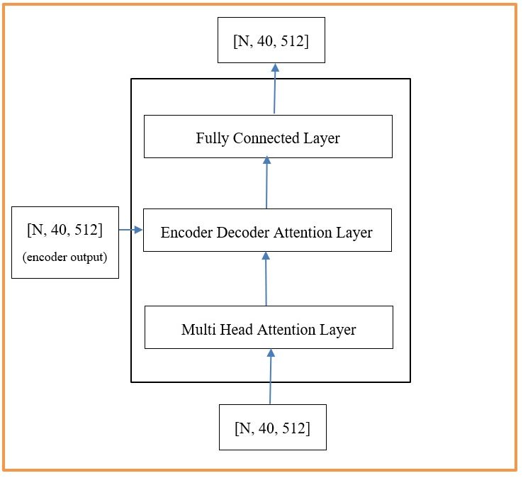
Here it might help to look at a diagram of the decoder layer.

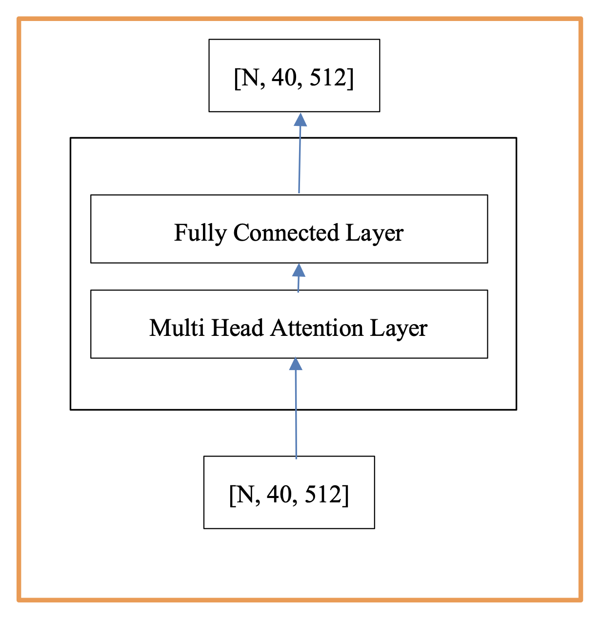
As can be seen we need a Multi-Head Attention layer followed by a FeedForward layer. Two normalizations (ln1, ln2) can also be performed.

class Block(nn.Module): def __init__(self, n_embd, n_head): ## (512, 8) super().__init__() head_size = n_embd // n_head ## 64 self.sa = MultiHeadAttention(n_head, head_size) self.ffwd = FeedForward( n_embd) ## 512 self.ln1 = nn.LayerNorm(n_embd) self.ln2 = nn.LayerNorm(n_embd) def forward(self, x): x = x + self.sa( self.ln1(x) ) x = x + self.ffwd( self.ln2(x) ) return x

The Block class uses 2 more classes which are Multi-Head Attention and FeedForward. We can now proceed to define these.
We can first define the Multi-Head class as follows

class MultiHeadAttention(nn.Module): def __init__(self, num_heads, head_size): ## (8, 64) super().__init__() self.heads = nn.ModuleList( [ Head(head_size) for _ in range(num_heads) ] ) self.proj = nn.Linear(n_embd, n_embd) ## 512, 512 self.dropout = nn.Dropout(dropout) def forward(self, x): out = torch.cat( [ h(x) for h in self.heads ], dim = -1 ) out = self.proj( out ) out = self.dropout( out ) return out

The Masked multi-head attention layer is done N\_head times (e.g. 8) in parallel and the results are concatenated. This concatenated result is added to the original after mapping it through one more layer and a Residual can also be used. The 2 key aspects are the instantiation of 8 heads which are parallel and independent of each other using "nn.ModuleList"as can be seen in the next code listing

self.heads = nn.ModuleList( [ Head(head_size) for _ in range(num_heads) ] )

and the concatenation of the 8 head Heads of size 64 to create a new tensor of size 512 ( 64 * 8 = 512).

out = torch.cat( [ h(x) for h in self.heads ], dim = -1 )

The FeedForward class is very straight forward as can be seen below. It is a simple linear layer followed by a non-linearity.

class FeedForward(nn.Module): def __init__(self, n_embd): ## 512 super().__init__() self.net = nn.Sequential( nn.Linear(n_embd, 4 * n_embd), ## [512, 4*512] nn.ReLU(), nn.Linear(4 * n_embd, n_embd), ## [4*512, 512] nn.Dropout(dropout), ) def forward(self, x): return self.net(x)

Finally, the Multi-Head Attention class use the Head class where the Attention mechanism is defined. The next code segment is probably the most important in terms of the power of Transformers. It defines the Attention layer. Here we define the Attention Head class.

class Head(nn.Module): def __init__(self, head_size): super().__init__() self.key = nn.Linear(n_embd, head_size, bias=False) ## [512, 64] self.query = nn.Linear(n_embd, head_size, bias=False) ## [512, 64] self.value = nn.Linear(n_embd, head_size, bias=False) ## [512, 64] tril_def = torch.tril( torch.ones(block_size, block_size) ) ## [40, 40] self.register_buffer( 'tril', tril_def ) self.dropout = nn.Dropout(dropout) def forward(self, x): B, T, E = x.shape ## [batch_size, 40, 512] k = self.key( x ) ## k = (B, T, 64) q = self.query( x ) ## q = (B, T, 64) E2 = 64 ## I think this is 64 and not 512 ## (B, T, E) @ (B, E, T) -> (B, T, T) wei = q @ k.transpose(-2, -1) * E2 ** -0.5 wei = wei.masked_fill( self.tril[:T, :T] == 0, float('-inf') ) ## (B, T, T) wei = F.softmax( wei, dim= -1 ) ## (B, T, T) wei = self.dropout( wei ) ## perform weighted aggregation of values v = self.value( x ) ## x = (B, 40, E) out = wei @ v ## (B, T, T) @ (B, T, 64) -> (B, T, 64) return out

The sentence and corresponding padding mask are the only inputs to this Attention layer. The output of this Attention mechanism is then passed to a fully connected layer. The mask must not be part of the computational graph since it is only used for masking. We use the following command to keep it out of the computational graph.

self.register_buffer('tril', torch.tril(torch.ones(block_size, block_size)))

The Attention mechanism uses K, Q, and V to compute the Attention scores. The values are computed from the original "x" input. The intuition is that the sentence is compared with itself and that is why the comparison or scores matrix will result in size [N_tokens, N_tokens] (e.g. [40, 40]). This is accomplished with the following code:

self.key = nn.Linear(n_embd, head_size, bias=False) ## [512, 64] self.query = nn.Linear(n_embd, head_size, bias=False) ## [512, 64] self.value = nn.Linear(n_embd, head_size, bias=False) ## [512, 64]

The input "x" is of size [N, 40, 512] and the "look_ahead_mask" is of size [N_batches, 40, 40]. Remember that using "nn.Linear" is equivalent to the following:

Wq = torch.tensor( [batch_size, 512, 64] ) bq = torch.tensor( [batch_size, 40, 64] ) Q = torch.matmul( x, Wq ) + bq # Nx40x64 Wk = torch.tensor( [batch_size, 512, 64] ) bk = torch.tensor( [batch_size, 40, 64] ) K = torch.matmul(x, Wk) + bk # Nx40x64 Wv = torch.tensor( xavier_init( [batch_size, 512, 64] ) ) bv = torch.tensor( torch.random_normal( [batch_size, 40, 64] ) ) V = torch.matmul(x, Wv) + bv # Nx40x64

Once Q, K, and V are defined, the next step is to multiply Q times K. You can think of this as calculating a score of the importance of "token_i" in "x" to all other words in "x".

## (B, T, 64) @ (B, E, 64) -> (B, T, T) wei = q @ k.transpose(-2, -1) * E ** -0.5 wei = wei.masked_fill( self.tril[:T, :T] == 0, float('-inf') ) ## (B, T, T) wei = F.softmax( wei, dim= -1 ) ## (B, T, T) wei = self.dropout( wei )

The variable "wei" is computed by a nn.matmul between Q and the transpose of K like so

wei = nn.matmul( Q, K, transpose_b=True)

This nn.matmul results in a matrix of size [N, 40, 40]. We then divide "wei" by

sqrt( Embd_size )

where Embd_size is equal to 64 (i.e. E ** -0.5). At this point "wei" continues to be of size [N, 40, 40]. The following code segment adds "wei" to the Mask.

wei = wei.masked_fill( self.tril[:T, :T] == 0, float('-inf') )

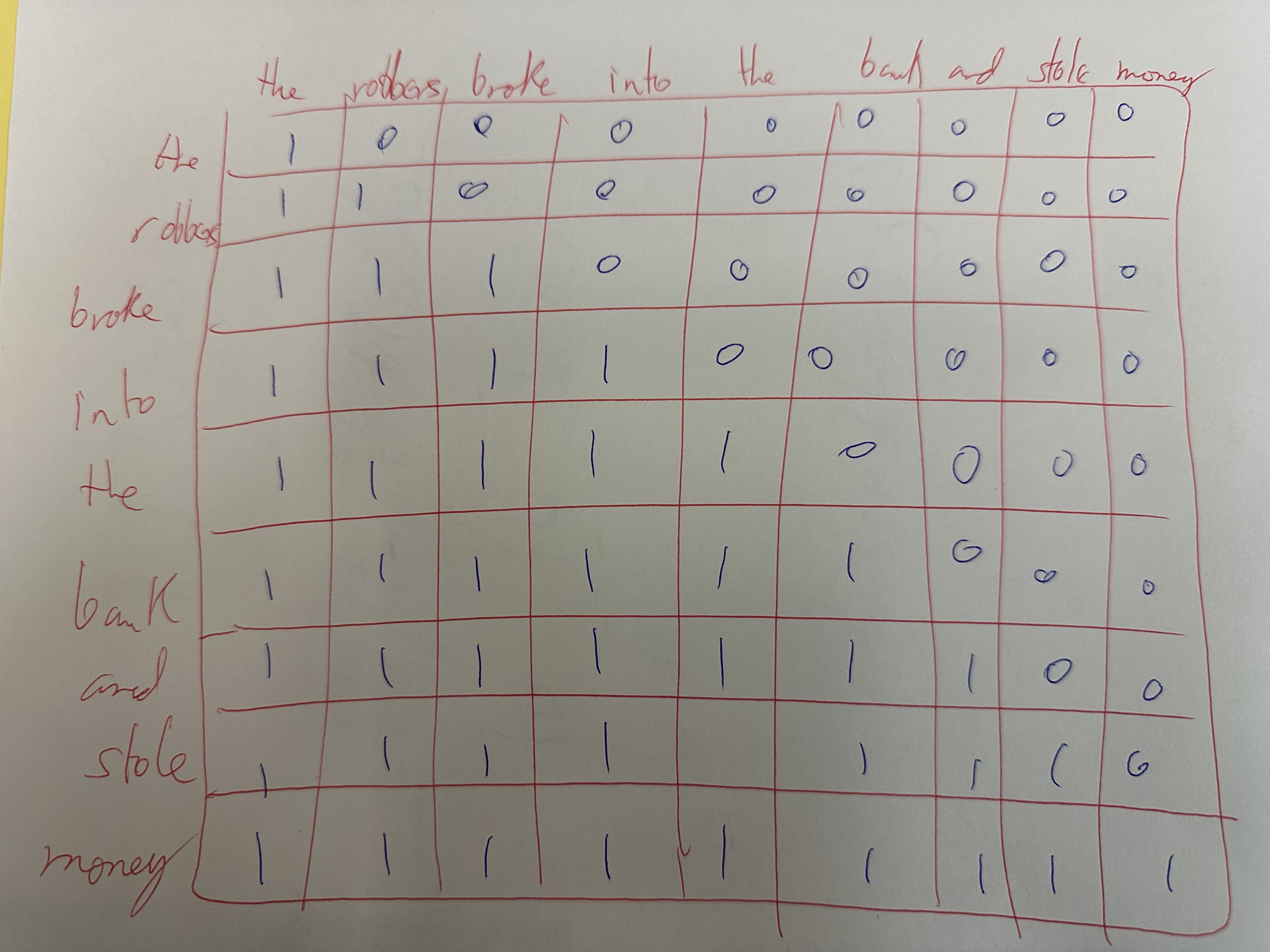
An example of the effect of the mask on one sample in the batch

The "look_ahead_mask" is of size [N, 40, 40]. This should be an addition of [N, 40, 40] + [N, 40, 40]. Notice that the wei.masked_fill function makes use on an infinity parameter. A simplified view of this operation is as follows:
wei = wei + (look_ahead_mask * -1e9)
The final part of the forward function in the Head class (next code segment) finishes the Attention computation. The softmax is used to normalize on the last axis so that the scores add up to 1 (axis -1 is for last dimension in the tensor).

class Head(nn.Module): ... def forward(self, x): ... ## (B, T, T) wei = F.softmax( wei, dim= -1 ) ## (B, T, T) wei = self.dropout( wei ) ## perform weighted aggregation v = self.value( x ) ## (B, T, E) out = wei @ v ## (B, 40, 40) @ (B, 40, 64) -> (B, 40, 64) return out

Finally, the following operation is performed which result in a tensor of size [N, 40, 64]. Remember that 8 of these Head output tensors will be concatenated to return to the original size of [N, 40, 512] (64 * 8 = 512).
out = nn.matmul(wei, V)
The operation looks like the following [N, 40, 40] * [N, 40, 64]. So, in summary you calculate the keys, queries, and values which are tensors that map the input \textbf{x} of size [N, 40, 512] to size [N, 40, 64]. We then calculate the scores matrix (wei) which is the Attention mechanism. This is a dot product. We matrix multiply Q with the transpose of K. This results in a matrix that is size [N, 40, 40]. After calculating the score matrix (wei), we need to mask the values so that we don’t cheat by looking ahead. We apply the look ahead and padding masks. The mask for look ahead attention happens before the softmax calculation. Notice that the masking is done to the dot_product scores matrix (wei) only. The mask is multiplied with -1e9 (close to negative infinity). This is done because the mask is summed with the scaled matrix multiplication of Q and K and is applied immediately before a softmax. The goal is to zero out padded cells, and large negative inputs to softmax are near zero in the output.

For example, the softmax ( torch.nn.softmax(a7) ) for “a” defined as follows:

a7 = torch.constant([0.6, 0.2, 0.3, 0.4, 0, 0, 0, 0, 0, 0])

gives the following

<torch.Tensor: shape=(10,), dtype=float32, numpy= array([0.15330984, 0.10276665, 0.11357471, 0.12551947, 0.08413821, 0.08413821, 0.08413821, 0.08413821, 0.08413821, 0.08413821], dtype=float32)>

now, if some of the values are negative infinities

b7 = torch.constant([0.6, 0.2, 0.3, 0.4, -1e9, -1e9, -1e9, -1e9, -1e9, -1e9])

then the softmax operation on b7 (torch.nn.softmax(b7)) should give us

<torch.Tensor: shape=(10,), dtype=float32, numpy= array([ 0.3096101 , 0.20753784, 0.22936477, 0.25348732, 0. ,0. , 0. , 0. , 0. , 0. ], dtype=float32)>

Notice the infinities are now zeros!
The decoder has a final linear layer after the 6 decoder_layer functions. The final layer in the decoder is the decoder_final_layer. This is a linear layer with no non-linearities and a softmax that maps the tensor [N, 40, 512] to a tensor of size [N, 40, n_vocab_size]. And that covers all the classes of the NN architecture. We are now ready to instantiate the GPT and call the core functions for the optimizer, etc. like so:

The linear algebra operations that make Attention work

I have further broken down all the previous linear algebra operations using random data into the linked jupyter notebook. I recommend going through it to further understand what is going on.

• Attention and linear algebra
• nn.Linear() as w, x, b, matmul
• Video

Instantiate the GPT

model = GPTModel() m = model.to(device) optimizer = torch.optim.Adam( m.parameters(), lr=learning_rate )

The training function is presented below and is straight forward

for iter in range(max_iters): if iter % eval_interval == 0: losses = estimate_loss() print(f"step {iter}: train loss {losses['train']:.4f}, val loss {losses['val']:.4f}") xb, yb = get_batch('train') ## eval the loss logits, loss = m(xb, yb) optimizer.zero_grad(set_to_none=True) ## zero out loss.backward() optimizer.step()

Now, regenerate after some training

## Starting token id_sos = 0 sos_context = torch.zeros( (1, 1), dtype=torch.long, device=device ) generated_text = m.generate(sos_context, max_new_tokens=500)[0].tolist() print( decode(generated_text) )

Using the generate function gives GPT generated text. Obviously, the amount of data will determine the quality of a GPT and it can take a lot of money and time to properly train a GPT. The following are examples of generated text using just single books or scripts.
For South Park training data we can get

Mr. Hankey: Who, don't look it, but looks like you have thrown them. These chees. Stan: Now back a friend people.me. Kenny: (HA f!) Stan: The new bestsays to expon is weep thing the beny first they wan t Stan: Thank you. Kyle: His realet! Stan, co musb me friends Vagisil magine? Stan: Nat Just sind out hurt. Hallway gaves millions? Are Me: Preest y revitalizing there? Stan: D'RCRANNSSEA. Stan: What? Stan: Dammit! Cartman: If anyone cools orget and have meet hundestly kids he since

For Harry Potter training data we can get

HARRY: What is saying that Time-Turner, ghe dangerous and gentlemen — GINNY: And is Albus Scorpius about to ldemborn King. And we should be very moths die. He means the rumble. It feels the appos his and forcement. HARRY: Get out out of the train is and for the Ministry had of fist or your pament. DRACO: Wh, does it say? HARRY: You came? RON enters on a baccused by through through, finality. It is it can’t better but Padma sets in for one champions and to be to reface the Boy — she speak. HARRY: Year the rumors? PROFESSOR McGONAGALL: I came it extraord the might be minty Iave progice to your paplay — then your nose? (She fining, an is hurts.) I, am Dad. Sound that . . . weld your have beyou’ve gone? SCORPIUS is saying in his roommount. What she falls talking about the blanked than I had a son. ALBUS: I’ll give to you that strave to do with my died it son. And my for you because it fly. And you schoolow how Harried in Potion

And that concludes the discussion on GPTs.

Encoder Only Models

The encoder has 6 sub-layers called encoder layers. Each encoding layer has a Multi-Head Attention layer followed by a standard fully connected feed forward layer. The input to the encoder goes through all these layers in the encoder and it is converted into an encoder output. The input to the encoder and the output of the encoder have the same dimensions. For instance, here, the input to the encoder would be the English sentence. The attention layer consists of 8 parallel Attention sub layers that are later concatenated. The intuition is that each of these 8 layers can learn something new and different. So this gives more capacity to the network. The input to the encoder goes through all these layers in the encoder and is converted into an encoder output. The next code segment shows the standard encoder architecture code. Notice it is almost exactly like the GPT (decoder) code. The only difference is in the last layer. The pure Encoder does not need to predict words. Instead, it takes sentences and converts them to embeddings. In this case of size [B, 40, 512].

class Encoder_Model(nn.Module): def __init__(self): super().__init__() self.token_embedding_table = nn.Embedding(vocab_size, n_embd) ## [65, 512] self.pos_emb_table = nn.Embedding(block_size, n_embd) ## [block, 512] self.blocks = nn.Sequential( *[ Block(n_embd, n_head=n_head) for _ in range(n_layer) ] ) self.ln_f = nn.LayerNorm( n_embd ) def forward(self, idx, targets=None): B, T = idx.shape ## (Batch, 40) ## ids and targets are both (B, T) tensors of integers tok_emb = self.token_embedding_table(idx) pos_emb = self.pos_emb_table(torch.arange(T, device=device)) x = tok_emb + pos_emb ## [B, T, E] or [64, 40, 512] ## This is the architecture x = self.blocks( x ) ## (B, T, E) x = self.ln_f( x ) ## (B, T, E) ## [B, 40, 512]

Notice that 6 identical encoder layers are created were the outputs of one become the inputs of the next layer. The dimensions of all inputs and output at this stage are the same [B, 40, 512] where B is batch size. The input is a batch of "B" sentences, with 40 tokens per each sentence, and where 512 is each id that has been embedded to a vector of size 512. Remember that the embedding vectors of size 512 are learned by the model so initially they are random data. We use a padding mask to ignore tokens with 0 value (i.e. padding). BERTs are based on the encoder part of the original Transformer, and are encoder only Transformers.

BERT

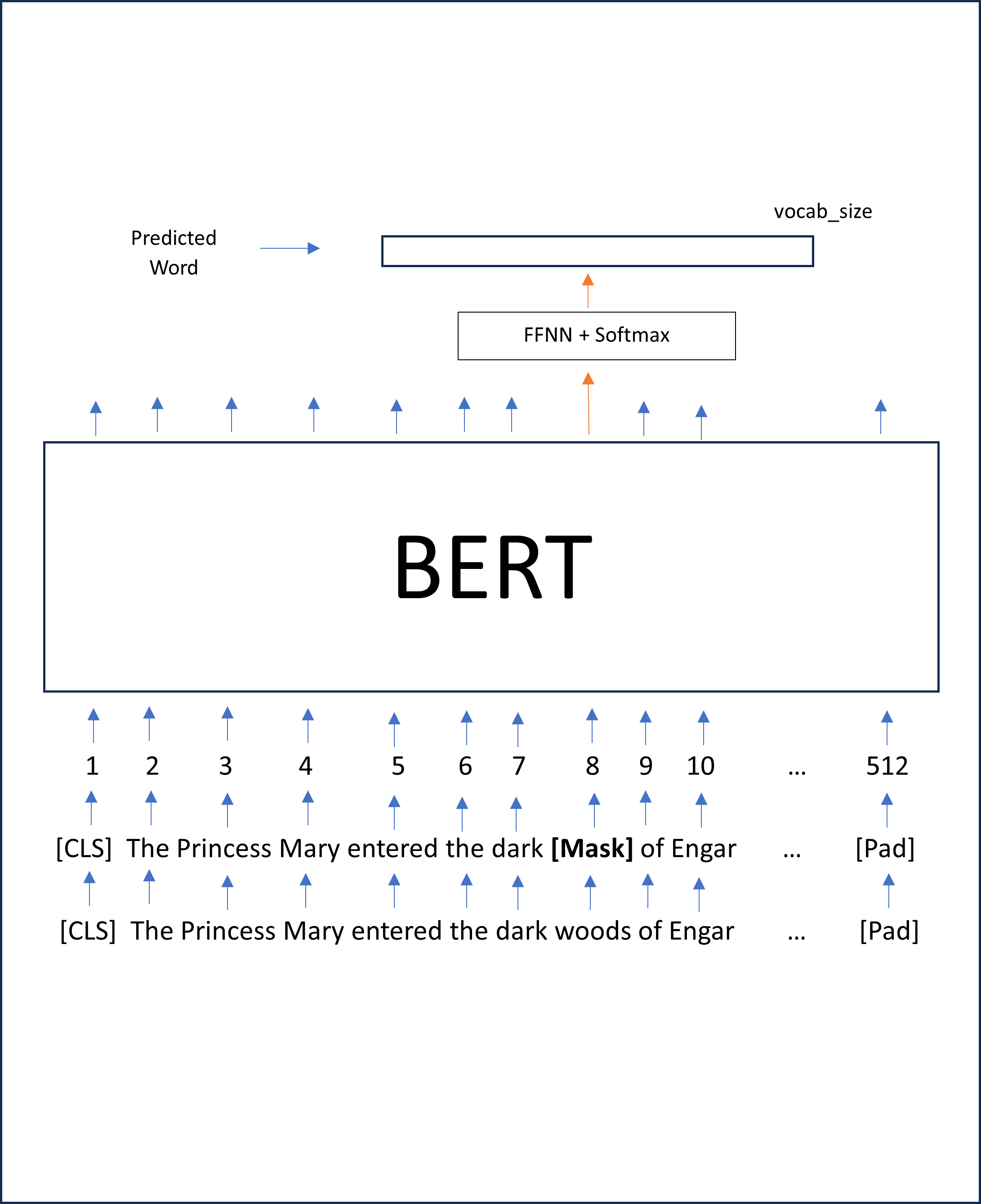
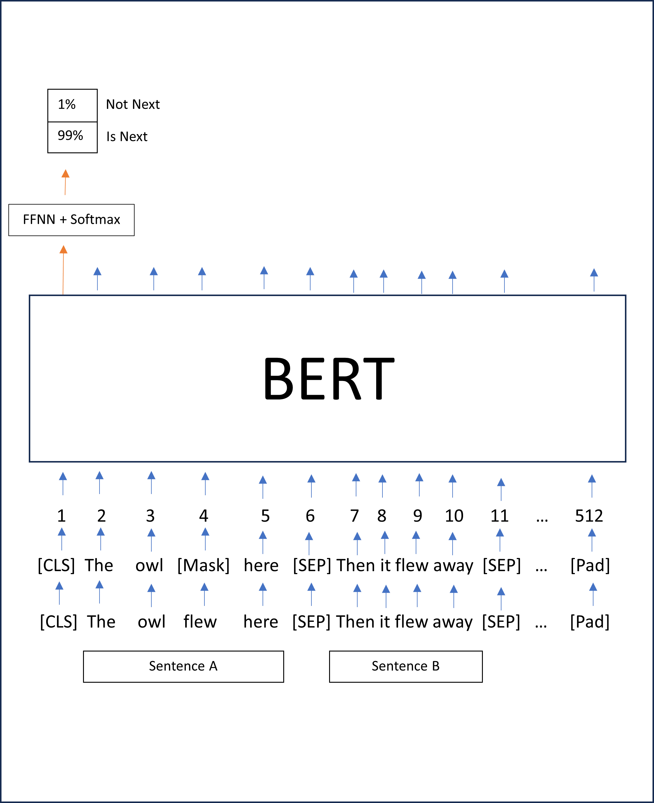
BERT is an example of an encoder-only Transformer. In contrast to pure Encoders that take a sentence and only produce an embedding (e.g. [B, 40, 512]), BERT models will add neural network layers (called heads) after the embedding (e.g. [B, 40, 512]) to convert those embeddings into words or sentences. BERT stands for Bidirectional Encoder Representations from Transformers. They were trained using 2 approaches.

The approaches are:

• Masked language task training
• Two sentence task training

The first task BERT was pre-trained on was the Masked Language modeling approach. This approach is summarized in the previous figure. Here the BERT model receives the same sentence as input and output. Some tokens are masked and the model needs to learn to predict those masked tokens during the training process. The second task BERT was pre-trained on is a 2 sentence classification task. The figure below summarizes this approach. Basically, here, 2 sentences are given to the BERT model as input. The model trains to predict if these 2 input sentences are sequential whcih means they are also related, or if they are not sequential and, therefore, unrelated. BERT was originally developed by Google and there have now been several other versions that were developed. They all follow the simliar naming convention of being called RoBERTa, AlBERT, DistilBERT, etc.

Encoder Decoder Transformers

In this section, I will discuss the first version of the Transformer first made popular in the paper “Attention Is All You Need” by Vaswani et al. They were first used for language translation. The Encoder Decoder with Multi Head Attention Transformer is a very deep network. The architecture has an encoder followed by a decoder. The decoder layer has 2 inputs. One input is the encoder output. The second input to the decoder varies based on whether you are training or predicting. If you are training, the input to the decoder is the sentence in the other language. For instance, the Spanish sentence. In the decoder, when training the Transformer, a mask is needed to prevent the model from seeing all the words it is trying to predict. This is called a look ahead mask. If you are testing, the input to the decoder is just the previous words before the word you are trying to predict. You start with a start of sentence token (e.g. ) and predict iteratively. The predicted word is then added to the previous tokens and the process is repeated. In the Encoder Decoder Transformer (for the language translation problem), the decoder layer has 2 inputs. One input is the encoder output. The second input to the decoder varies based on whether you are training or predicting. If you are training, the input to the decoder is the sentence in the other language. For instance, the Portuguese or Spanish sentence. When training, a mask is needed here to prevent the model from seeing all the words it is trying to predict. This is called a look ahead mask. If you are testing, the input is just the previous words before the word you are trying to predict. You start with a start of sentence token (e.g. ) and predict. The predicted word is then added to the previous tokens and the process is repeated. The decoder consists of 6 decoder layers, followed by a linear layer. Each decoder layer has a decoder multi-head attention layer, followed by a decoder-encoder attention layer, and a fully connected layer. The decoder architecture for the Encoder Decoder Transformer (for the language translation problem) can be seen in the following figure.

The attention layers consist of 8 parallel attention sub layers that are later concatenated. The numbers 6 and 8 are a choice the architect makes. The first code segment in this section describes the decoder’s overall architecture. The decoder has more inputs than the encoder. The decoder_layer is the busiest function of the Transformer. It is basically very similar to the encoder_layer except that it has 2 attention mechanisms instead of just one. The Multi-Head Attention is the first attention mechanism. For our reference language problem, The Portuguese sentence and corresponding padding mask are the only inputs to this sub layer. The output of this attention mechanism plus the encoder output are the inputs to the second attention mechanism which is usually referred to as the Encoder-Decoder-Attention mechanism. The output of this second Attention mechanism is passed to a fully connected layer just like the one used in the encoder. The first Masked multi-head attention layer is done 8 times in parallel just like in the encoder and the results are concatenated. This concatenated result is added to the original after mapping it through one more layer to calculate the residual. The final layer maps a tensor of size [N, 40, 512] to a tensor of size [N, 40, pt_vocab_size] where pt_vocab_size is the size of the Portuguese vocabulary. This is what allows us to select the predicted word.

Data Wrangling from Scratch

PyTorch offers many new techniques for extracting and processing data sets. As I like building things from scratch, I will present my own approach to data wrangling for Transformers. The approach is very standard and is similar to what you do in NLP for algorithms like word2vec, for instance. For this example, I will use the implementation of a Transformer-based Translator using the English to Portuguese dataset. The code and data set are available on the book GitHub. First, let us import the libraries:

import sklearn import numpy as np import nltk from nltk.tokenize import word_tokenize from numpy import genfromtxt from sklearn import datasets from sklearn.model_selection import train_test_split import pandas as pd import pickle import collections

I like working with python dictionaries so, for this example, I extracted the data set and created python dictionaries for training and testing. I saved the dictionaries to Python pickle files for ease of use. The following code shows how to load the dictionaries.

def load_dictionary(file_name): with open(file_name, 'rb') as handle: dict = pickle.loads( handle.read() ) return dict

After loading the data sets from file, you have to create the dictionary and reverse dictionary. You create 2 dictionaries per language (e.g. two for English and two for Portuguese). These are dictionaries of ids to tokens and vice-cersa. Notice that I set the vocabulary size to 12,000. You can play with this value for optimal performance.

## Includes <eos> and <sos> tokens def build_dataset(words): START_TOKEN = "<sos>" END_TOKEN = "<eos>" UNK_TOKEN = "<unk>" count = collections.Counter(words).most_common(12000) dictionary = dict() for word, _ in count: ##add + 1 so that 0 is not used as index to avoid padding conflict dictionary[word] = len(dictionary) + 1 ## + 1 size_vocab = len(dictionary) dictionary[START_TOKEN] = size_vocab dictionary[END_TOKEN] = size_vocab + 1 dictionary[UNK_TOKEN] = size_vocab + 2 reverse_dictionary = dict(zip(dictionary.values(), dictionary.keys())) return dictionary, reverse_dictionary

The following is an example function in case you want to process sentences with regular expressions or tokenize manually.

def preprocess_sentence(sentence): sentence = sentence.lower().strip() # creating a space between a word and the punctuation following it # eg: "it is a cat." => "it is a cat ." sentence = re.sub(r"([?.!,])", r" \1 ", sentence) sentence = re.sub(r'[" "]+', " ", sentence) # replacing everything with space except (a-z, A-Z, ".", "?", "!", ",") sentence = re.sub(r"[^a-zA-Z?.!,]+", " ", sentence) sentence = sentence.strip() return sentence

For tokenization, I used the NLTK tokenizer. In the paper “Attention Is All You Need”, the authors used byte pair encoding. Byte pair encoding does not use full words as tokens. Instead, you do something like this: "walk" and "ing" for the word “walking”. Therefore, words are broken into smaller elements (subwords). Byte-pair encoding is used to tokenize sentences in a language, which, like the WordPiece encoding, breaks words up into tokens that are slightly larger than single characters but less than entire words.

def get_tokens(sentence_list): tokens_list = [] for sentence in sentence_list: tokens = word_tokenize(sentence) for word in tokens: tokens_list.append(word) tokens_list = np.array(tokens_list) return tokens_list

Once you have the dictionaries and the tokens, you can proceed to convert words into ids with the encode function.

def encode(sentence, dictionary): ids_list = [] tokens = word_tokenize(sentence) for word in tokens: if word in dictionary.keys(): ids_list.append( dictionary[word] ) return ids_list

Decoding is just the process in reverse. Here you convert ids back to tokens using the reverse dictionary for convenience and speed up.

def decode(list_ids, reverse_dictionary): words_list = [] for id in list_ids: if id in reverse_dictionary.keys(): words_list.append( reverse_dictionary[id] ) return words_list

The following function aligns the English and Portuguese sentence pairs and creates two lists.

## this returns 2 lists of english and portuguese sentences ## that are aligned by index def get_en_and_pt_sentences(train_dict): en_list, pt_list = [], [] for key, val in train_dict.items(): print(key) print(val) en_list.append( val['en'] ) pt_list.append( val['pt'] ) return en_list, pt_list

The below line of code just loads the sentences data before processing from the pickle objects.

## Read in the data of english and portuguese sentences train_dict = load_dictionary("data/en_pt_train_dictionary.txt") validation = load_dictionary("data/en_pt_val_dictionary.txt" )

The next function creates 2 lists of aligned English and Portuguese sentences.

english_sentence_list, portuguese_sentence_list = get_en_and_pt_sentences(train_dict)

The function get_tokens converts each sentence into a list of tokens.

print("creating the dictionaries takes a while ... ") en_tokens = get_tokens(english_sentence_list ) pt_tokens = get_tokens(portuguese_sentence_list)

After creating the dictionaries for each language, we calculate the vocabulary size for each language.

## when 2 languages, you have 2 separate tokenizers. en_dictionary, en_reverse_dictionary = build_dataset(en_tokens) pt_dictionary, pt_reverse_dictionary = build_dataset(pt_tokens) VOCAB_SIZE_EN = len(en_dictionary) VOCAB_SIZE_PT = len(pt_dictionary) print("vocab size english ", VOCAB_SIZE_EN) print("vocab size portuguese ", VOCAB_SIZE_PT)

The following “for” loop brings all the previous functions together. It results in 2 lists of sentence ids, one for each language (2 lists of Numpy objects). Notice that, to each sentence list of ids, we add the start token id at the beginning and the end token id at the end. The final “if” statement is used to only include sentences shorter than 40 tokens (the max length I used). Sentences shorter than 40 will be padded but all sentences will eventually be tensors of size 40 (n_tokens + padding).

english_sentence_ids_list = [] portuguese_sentence_ids_list = [] for i in range( len(english_sentence_list) ): en_sentence = english_sentence_list[i] pt_sentence = portuguese_sentence_list[i] en_sentence_ids = encode(en_sentence, en_dictionary) pt_sentence_ids = encode(pt_sentence, pt_dictionary) en_sentence_ids = np.array(en_sentence_ids) pt_sentence_ids = np.array(pt_sentence_ids) en_START_TOKEN_id = en_dictionary['<sos>'] en_END_TOKEN_id = en_dictionary['<eos>'] pt_START_TOKEN_id = pt_dictionary['<sos>'] pt_END_TOKEN_id = pt_dictionary['<eos>'] en_sentence_ids = np.concatenate( [ [en_START_TOKEN_id], en_sentence_ids, [en_END_TOKEN_id] ] ) pt_sentence_ids = np.concatenate( [ [pt_START_TOKEN_id], pt_sentence_ids, [pt_END_TOKEN_id] ] ) if len(en_sentence_ids) <= MAX_LENGTH and len( pt_sentence_ids) <= MAX_LENGTH: english_sentence_ids_list.append( en_sentence_ids) portuguese_sentence_ids_list.append( pt_sentence_ids)

Now we need to use a Torch padding function.

en_MAX_LENGTH = MAX_LENGTH pt_MAX_LENGTH = MAX_LENGTH + 1 english_sentence_ids_list = torch.preprocessing.sequence.pad_sequences( english_sentence_ids_list, maxlen=en_MAX_LENGTH, padding='post') portuguese_sentence_ids_list = torch.preprocessing.sequence.pad_sequences( portuguese_sentence_ids_list, maxlen=pt_MAX_LENGTH, padding='post')

If you would like to view the data, you can do so with the following code.

for i in range( len(english_sentence_ids_list) ): print("@@@@@@@@@@@@@@@@@@@@@@@@@@@") print(english_sentence_ids_list[i]) print(portuguese_sentence_ids_list[i]) ## input()

After padding, the data will look like this:

en [12110 203 4 3947 29 2 168 2 4 27 68 4333 8 3622 2943 1012 1 12111 0 0 0 0 0 0 0 0 0 0 0 0 0 0 0 0 0 0 0 0 0 0 ] pt [12210 13 4 3947 29 2 5 32 36 16 1145 4 58 34 7905 58 25 28 354 2482 3 17 27 28 4395 9 2886 7 12211 0 0 0 0 0 0 0 0 0 0 0 ]

And without padding, the data will look like this:

en [12110 13 4 3947 29 2 5 32 36 16 1145 4 58 34 7905 58 25 28 354 2482 3 17 27 28 4395 9 2886 7 12111 ] pt [12210 62 585 132 202 4395 11969 3 43 18 27 107 7042 15 10 814 11717 4 4053 89 2960 2 157 119 1 12211 ]

Summary

In this chapter, I have introduced the topic of Transformers. I discussed the main ideas and code for the Encoder Decoder with Multi-Head Attention Transformer first introduced by Vaswani et al. (2017), ideas of BERTs, and the GPT.