Chapter 2 - Traditional Machine Learning

In this chapter, I will address some of the general machine learning topics. I will use python, numpy, and the Sklearn library to provide example code on how to use the different models and other tools. I will quickly move through logistic regression to arrive at other algorithms. Much of what we learn from using the SKlearn kit can be integrated with PyTorch to make your deep learning code more powerful and modular. That way, you will be able to re-use your code for many different tasks. I will not focus on the theory of machine learning algorithms. There are many books on the theory of machine learning algorithms so instead I will concentrate on the practical aspects of using them in Python.

Copyright and License

Copyright © by Ricardo A. Calix.
All rights reserved. No part of this work may be reproduced or transmitted in any form or by any means, without written permission of the copyright owner.
License: MIT.

FTC and Amazon Disclaimer

This post/page/article includes Amazon Affiliate links to products. This site receives income if you purchase through these links. This income helps support content such as this one.

Traditional Machine Learning

In this chapter, I will address some of the general machine learning topics. I will use python, numpy, and the Sklearn library to provide example code on how to use the different models and other tools. I will quickly move through logistic regression to arrive at other algorithms. Much of what we learn from using the SKlearn kit can be integrated with PyTorch to make your deep learning code more powerful and modular. That way, you will be able to re-use your code for many different tasks. I will not focus on the theory of machine learning algorithms. There are many books on the theory of machine learning algorithms so instead I will concentrate on the practical aspects of using them in Python. Machine Learning (ML) is essential for automated systems to make decisions and to infer new knowledge about the world. This section describes some of the most important traditional methodologies currently in use in the field of machine learning. Machine learning approaches can be divided into supervised learning (such as Support Vector Machines) and unsupervised learning (such as K-means clustering). Within supervised approaches, the learning methodologies can be divided based on whether they predict a class or a magnitude, into classification and regression models, respectively. An additional categorization for these methods depends on whether they use sequential or non-sequential data. Classifiers are machine learning approaches that produce as an output a specific class given some input features. Important classifiers include Support Vector Machines (Burges 1998) commonly implemented using LibSVM (Chang and Lin, 2001), Naïve Bayes, artificial neural networks, deep learning based neural networks, decision trees, random forests, and the k-nearest neighbor classifier ( wittenRef ). Regression models are those that produce a real valued number instead of class such as the price or square footage of a house. In their simplest form, deep learning based methods are simply neural nets with more layers. Deep learning methods have made a big impact in the field of machine learning in recent years. In particular, they are very important because, given enough computational power, they can automatically learn the optimal features to be used in a ML model. In the past, learning what features to use required using humans to engineer the features. This issue has now been alleviated somewhat by deep learning. Additionally, artificial neural networks are models that can handle non-linearly separable data. In theory, this capability allows them to model data that may be more difficult to infer.

Code Issues

Before we begin, I want to address some issues about the code. First, I have tried to be consistent with other programmers of machine learning in Python. We will be using many libraries to implement the models. In particular, I selected to use the SKlearn library since it is very powerful and widely use. In general, I only introduce enough SKlearn code for us to know how to integrate it with PyTorch in our deep learning endeavors. For a more in-depth discussion of SKlearn, I highly recommend the book “Python Machine Learning” by Sebastian Raschka. I have tried to be consistent with the conventions used in that book so that both books can be used together. So now, getting back to the code, here is an example of some of the most important libraries that we can use for our machine learning code.

import numpy as np from sklearn import datasets from sklearn.cross_validation import train_test_split from sklearn.preprocessing import StandardScaler from sklearn.metrics import accuracy_score from matplotlib.colors import ListedColormap import matplotlib.pyplot as plt from sklearn.metrics import confusion_matrix from sklearn.metrics import precision_score from sklearn.metrics import recall_score, f1_score import pandas as pd from sklearn.preprocessing import LabelEncoder from sklearn import decomposition

As you may imagine the SKlearn library is the main library which contains most of the traditional machine learning tools we will discuss in this chapter. The numpy library is essential for efficient matrix and linear algebra operations. For those with experience with MatLab, I can say that numpy is a way of performing linear algebra operations in python similar to how they are done in MatLab. This makes the code more efficient in its implementation and faster as well. The datasets library seen above helps to obtain standard corpora. You can use it to obtain annotated data like Fisher’s iris data set, for instance. From sklearn.cross_validation we can import train_test_split which is used to create splits in a data matrix such as 70 percent for training purposes and 30 percent for testing purposes. From sklearn.preprocessing we can import the StandardScaler module which helps to scale data. We will use functions such as these to scale our data for the PyTorch based models. Deep learning algorithms can improve significantly when data is properly scaled. So, it is recommended to do this. We will use the sklearn.metrics module for performance evaluation of the classifiers. I will show that this module can be used with SKlearn models and with PyTorch models. Again, this will help to more easily understand deep learning since we don’t have to use the more complex and very verbose PyTorch functions.
The main metrics used for classification models are:

• accuracy_score
• recall_score
• f1_score
• precision_score
• confusion_matrix

The main metrics used for regression models are:

• coefficient of determination ($ R^2 $)
• RMSE

Two more very important libraries are matplotlib.pyplot and pandas. The matplotlib.pyplot library is very useful for visualization of data and results, and the pandas library is very useful for pre-processing. The pandas library can be very useful to pre-process large data sets in very fast and very efficient ways. There are some parameters that are sometimes useful to set in your code. The code sample below shows the use of np.set\_printoptions. The function is used to print all values in a numpy array. This can be useful when trying to visualize the contents of a large data set.

## set parameters np.set_printoptions(threshold=np.inf) ## print all values in numpy array

Let us assume that our data is stored in the matrix X. The code segment below uses the function train_test_split. This function is used to split a data set (in this case X) into 4 sets which are X_train, X_test, y_train, y_test. These are the 4 sets that will be used by the traditional or the deep learning models. The sets that start with X hold the data (feature vectors) and the sets that start with y hold the labels per sample (e.g. $ y_1 $ for the first feature vector, $ y_2 $ for the second feature vector, and so on). The values test_size=0.01 and random_state=42 in the function are parameters that define the split. The value 0.01 makes a train set that has 99 percent of all samples while the test set has 1 percent of all samples. In contrast test_size=0.20 would mean that there is a 80% and 20% split. The random_state=42 allows you to always get the same random data since the seed is defined as 42.

X_train, X_test, y_train, y_test = train_test_split(X, y, test_size=0.30, random_state=48) ## k-folds cross validation all goes in train sets (hence 0.01) X_train, X_test, y_train, y_test = train_test_split(X, y, test_size=0.01, random_state=42)

To call all the functions or models you can employ the following approach. Here we have defined 5 common models. Notice that each one gets the 4 data sets obtained from the percentage split. Notice also that the data files have a _normalized added to their name. This is a good standard approach used by programmers to indicate that this data has been scaled. The next chapter addresses scaling. Here you run X\_train through a scaler function to obtain X_train_normalized. The labels (y) are not scaled, in this case.

logistic_regression_rc(X_train_normalized, y_train, X_test_normalized, y_test) svm_rc(X_train_normalized, y_train, X_test_normalized, y_test) random_forest_rc(X_train, y_train, X_test, y_test) knn_rc(X_train_normalized, y_train, X_test_normalized, y_test) multilayer_perceptron_rc(X_train_normalized, y_train, X_test_normalized, y_test)

Before we talk about the models, let us address performance evaluation. Performance evaluation will help you to determine how good your classifier is given an annotated test data set.

Object Oriented Programming

Object oriented programming will be used extensively in this book to implement our deep learning algorithms. As is necessary with progress, the algorithms are more complicated, with deeper and more resource intensive networks. This is best exemplified by one of the newest deep learning algorithms: The Transformer. The algorithms are much more complicated. A little bit too much in fact and the programming languages are starting to abstract too much of the code. I have found that a simple solution to this was to write everything in an object oriented fashion. This way you are still defining the classes from scratch but you can also build far more complicated algorithms thanks to traditional object oriented programming techniques. A GPT can nicely be built with a reasonable amount of lines of code if leveraging object oriented programming techniques.
The following code segment includes a simple example of a class format we will use extensively throughout this book.

class LinRegNet(nn.Module): ## init the class def __init__(self): super().__init__() self.linear1 = nn.Linear(11, 1) ## perform inference def forward(self, x): y_pred = self.linear1(x) return y_pred

Performance Evaluation

As previously stated, performance evaluation depends on whether we are doing classification or regression.

Regression Performance Evaluation

The main metrics used for regression models are:

• coefficient of determination ($ R^2 $)
• RMSE

The most important regression evaluation metric is $ R^2 $. The range goes from 0-1 and 1 means that you have a good model. Generally, I have used sklearn metrics to evaluate regression models. The code can be seen in the following code listing:

## coefficient of determination (R**2) from sklearn.metrics import r2_score print( r2_score( y_pred.detach().numpy(), y_test.numpy() ) )

Classification Performance Evaluation

The main metrics used for classification models are:

• accuracy_score
• recall_score
• f1_score
• precision_score
• confusion_matrix

Evaluation of the performance of your classifiers is extremely important. The SKlearn kit provides very good modules to address this issue. In particular, evaluation often involves measuring accuracy, precision, recall, and f-measure. The best way to understand these metrics is to think of a confusion matrix. Confusion matrices show how many elements from a class are correctly and incorrectly classified.
For example, take the following:

Given this table, we can calculate accuracy as

$ accuracy = (a+d) / (a + b + c + d) $

precision is

$ precision = a / (a + c) $

the recall metric can be computed as follows

$ recall = a / (a + b) $

Finally, the f measure which is a harmonic average of recall and precision can be computed as follows

$ F = (2 * (precision*recall)) / (precision + recall) $

The sample code to obtain these metrics is provided below.

from sklearn.metrics import confusion_matrix from sklearn.metrics import precision_score, recall_score, accuracy_score, f1_score def print_metrics_function(y_test, y_pred): print('Accuracy: %.2f' % accuracy_score(y_test, y_pred)) confmat = confusion_matrix(y_true=y_test, y_pred=y_pred) print("Confusion Matrix:") print(confmat) print('Precision: %.3f' % precision_score(y_true=y_test, y_pred=y_pred, average='weighted')) print('Recall: %.3f' % recall_score(y_true=y_test, y_pred=y_pred, average='weighted')) print('F1-measure: %.3f' % f1_score(y_true=y_test, y_pred=y_pred, average='weighted'))

The code above shows a function to print the performance metric statistics. Notice that two sets are provided which are y_pred and y_test. The y_test data set contains the original annotated labels. The y_pred data set contains the labels predicted by your classifier. Each of the metric functions such as "f1_score" and "recall_score" uses these 2 data sets to calculate the respective metric.

Plotting Performance

In the following code segment we can see the function plot_metric_per_epoch() which can be used to plot metric value every N values. For this to work, you store the metric values in a list such as precision_scores_list and then proceed to plot these values using the matplot library.

def plot_metric_per_epoch( precision_scores_list ): x_epochs = [] y_performance= [] for i, val in enumerate(precision_scores_list): x_epochs.append(i) y_performance.append(val) plt.scatter(x_epochs, y_performance,s=50,c='lightgreen', marker='s', label='score') plt.xlabel('epoch') plt.ylabel('score') plt.title('Score per epoch') plt.legend() plt.grid() plt.show()

The output should look like the following figure.

Optimization

Before we begin to discuss some of the machine learning algorithms, I should say something about optimization. Optimization is a key process in machine learning. Basically, any supervised learning algorithm needs to learn a prediction equation given a set of annotated data. This prediction function usually has a set of parameters that must be learned. However, the question is “how do you learn these parameters?”

The answer is that you do so through:

optimization

In its simplest form, optimization consists of trying a set of parameters with your model and seeing what result they give you. If the result is not good, the optimization algorithm needs to decide if you should decrease the values of the parameters or increase the values of the parameters.

In general, you do this in a loop (increasing and decreasing) until you find an optimal set of parameters. But one of the questions to answer here is: do the values go up or down? Well, as it turns out, there are methodologies based on calculus that help you to make this decision.

Let us try to picture this with a graph (below).

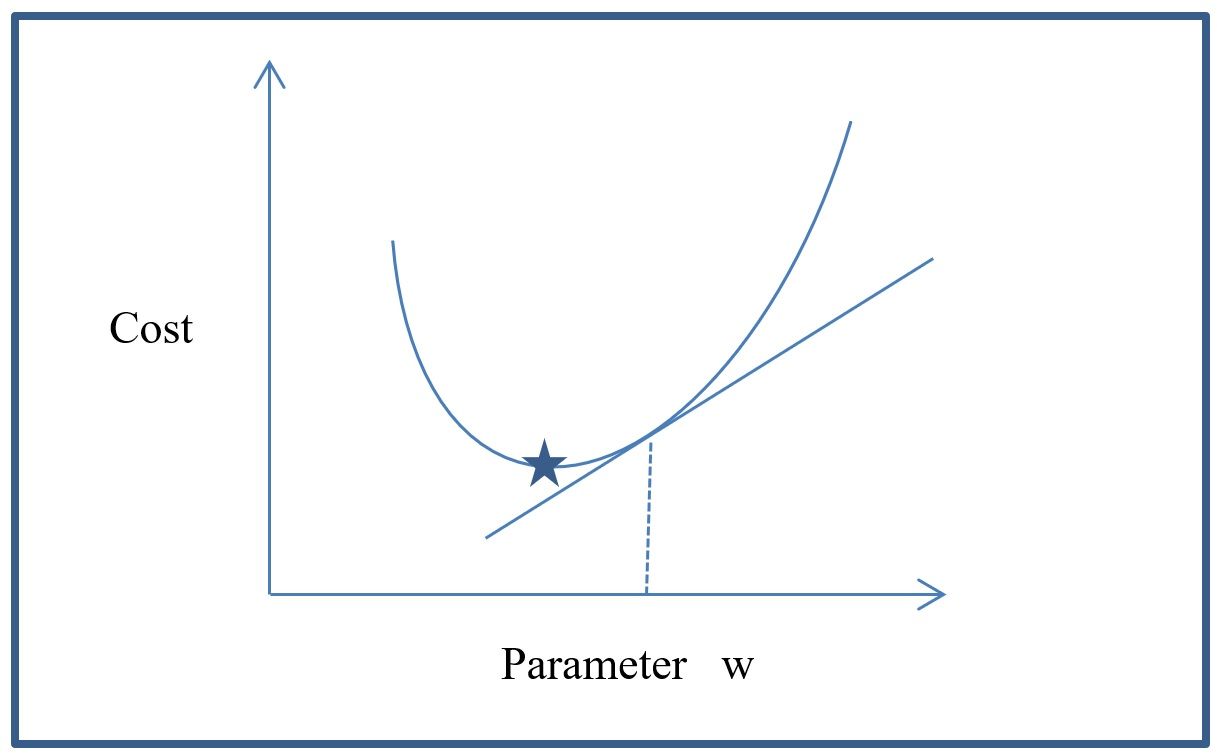
The above graph represents an optimization problem. The y axis represents the cost (or penalty) of using a given parameter. The x axis represents the value of the parameter (w) being used at the given iteration. The curve represents the behavior that the function being used to minimize the cost will follow for every value of parameter w.

As shown in the graph, the optimal value for the curve is found where the star is located (i.e where the value of cost is at a minimum). So, somehow the optimization algorithm needs to travel through the function and arrive at the position indicated by the star.

At that point, the value of “w” reduces the cost and finds the best solution. Instead of trying all values of “w” at random, the algorithm can make educated guesses about which direction to follow (up or down). To do this, we can use calculus to calculate the derivative of the function at a given point. This will allow us to determine the slope at that point. In the case of the graph, this represents the tangent line to the curve if we calculate the derivative at point w. If we calculate the slope at the position of the star symbol, then the slope is zero because the tangent at that point is parallel to the x axis. The slope at the point “w” will be positive. Based on this result, we can tell the direction we want to take for parameter w (decrease or increase). This type of optimization is called gradient descent and is very important in machine learning and deep learning. There are several approaches to implement gradient descent and this is just the simplest explanation for conceptual purposes. We can write the algorithm for this technique as follows:

old_x = 0 new_x = 4 step_size = 0.01 precision = 0.00001 def function_derivative(x): return 3*x ** 2 – 6*x while absolute_value(new_x – old_x) > precision: old_x= new_x new_x = old_x – step_size * function_derivative(old_x) print(“result is: ”, new_x)

In the previous code example we assume a function of

$ f() = x^3 - 3 x^2 + 7 $

that needs to be optimized for parameter x. We will need the value of the derivative for each point x. The derivative for f() is:

$ f '() = 3 x^2 - 6x $

So, the parameter x can be calculated in a loop using the derivative function which will determine the direction to follow when increasing or decreasing the parameter x.

Logistic Regression

Logistic regression is a simple algorithm that is often used by practitioners of machine learning because it can obtain good results. Logistic regression is a linear function much like linear regression which predicts the probability of a sample belonging to a given class. Logistic regression uses another optimization function instead of the standard least squares cost function used in linear regression.

def logistic_regression_rc(X_train_normalized, y_train, X_test_normalized, y_test): from sklearn.linear_model import LogisticRegression lr = LogisticRegression(C=1000.0, random_state=0) lr.fit(X_train_normalized, y_train) y_pred = lr.predict(X_test_normalized) print_stats_percentage_train_test( "log re", y_test, y_pred)

The predicted values from a standard regression approach are now passed through a sigmoid function that basically maps the output to a probability range scale between 0 and 1. The code below provides an example of how to use the logistic regression function with SKlearn. Later, we will implement this logistic regression function again with PyTorch. In the previous function, the train and test sets are provided for the model to be trained and tested. In SKlean most steps are abstracted. In contrast, PyTorch will allow us to define more steps such as the cost function, optimization, and inference equation and other aspects. In the function logistic_regression_rc, first you initialized a logistic regression object (lr) and then you train and test it with the functions lr.fit and lr.predict. The final step is to measure performance using the previously described function print_stats_percentage_train_test. Most classifiers are implemented in the same way with SKlearn. In the next section, I will demonstrate how this is done for a neural network in Sklearn.

Neural Networks

Neural networks are very complex systems that take a long time to train. Therefore, the use of them in SKlearn may not be recommended except for the smallest of data sets. The code is shown here for contrast purposes with later implementations of neural networks in PyTorch. In the next chapters, we will focus on how to do this in PyTorch and how to create networks of multiple layers.


In the code below we can see that everything is very similar to the previous logistic regression implementation. The new changes appear in the definition of the clf multilayer object. Here, the parameter hidden_layer_sizes=(100,100) means that the architecture of the network consists of 2 hidden layers with 100 neurons each. A parameter such as (200, ) would mean that the network has 1 hidden layer with 200 neurons.

def multilayer_perceptron_rc(X_train_normalized, y_train, X_test_normalized, y_test): from sklearn.neural_network import MLPClassifier clf = MLPClassifier(solver='lbfgs', alpha=1e-5, hidden_layer_sizes=(100,100), random_state=1) clf.fit(X_train_normalized, y_train) y_pred = clf.predict(X_test_normalized) print_stats_percentage_train_test("multilayer perceptron", y_test, y_pred)

KNN

The k-nearest neighbor (KNN) classifier is a popular algorithm that I always like to use. It requires very little parameter tuning and can be easily implemented. Here, the code is implemented in mupy becasue of its simplicity. The n_neighbors parameter is the k. In this case, the k closest samples are selected.

In the next code listing, you can see all the code needed to run KNN. Wow! Pretty short right? This code splits our data into "train" and "test" sets. Then grabs every sample in the test set and compares it to every sample in the train set. For each test sample, we get all distances between the test samples and all train samples. We then rank them and select the top "K" distances. Finally, we assign the majority class associated for the top 5 distances. That is it!

import numpy as np import pandas as pd import matplotlib.pyplot as plt import matplotlib.tri as tri From pyodide.http import open_url def euclidean_distance(v1, v2): return np.sqrt( np.sum( (v1 - v2)**2 ) ) def predict(test_x): k = 5 distances = [ euclidean_distance(test_x , x) for x in X_train ] k_neighbor_indices = np.argsort(distances)[:k] labels = [ y_train[i] for i in k_neighbor_indices ] labels_np = np.array( labels ) pred = int( np.mean(labels_np) ) return pred url1 = ("https://rcalix1.github.io/Build-Fun-AI-Projects-that-Run-on-the-Web/volume-1-pyscript-and-knn/chapter3/knn/iris.csv") iris_pd = pd.read_csv(open_url(url1)) iris_pd['species'] = iris_pd['species'].replace({'setosa':0, 'versicolor':1 , 'virginica':2}) iris_np = iris_pd.to_numpy() np.random.shuffle(iris_np) X_train = iris_np[1:130, :4] y_train = iris_np[1:130, 4] X_test = iris_np[130:150, :4] y_test = iris_np[130:150, 4] def my_gen_function(): accum_res = "" for i, test_x in enumerate( X_test ): the_pred = predict(test_x) my_gen_function()

The next code segment includes a function called the Euclidean distance as can be seen in the next code listing.

def euclidean_distance(v1, v2): return np.sqrt( np.sum( (v1 - v2)**2 ) )

This is the function that measures the distance between 2 points in a vector space. These 2 point need to have the same size but the size can be of any dimension. For instance, for our Iris data, every point has 4 features. So in the code the 2 points v1 and v2 would be of size 4 each. However, we could also have points (samples) of many more dimensions. For instance, points with 100 features. So in this case v1 and v2 would both need to have size 100. But the cool thing is that the function for distance calculation would still work. That is the power of Numpy.

The name Euclidean distance comes from a Greek philosopher named Euclid. He is best known for putting together one of the earliest books on geometry. The book was so good for its time that the type of mathematics it discussed became known as Euclidean geometry.

So, where does this magical Euclidean distance function come from? Would you believe that it is related to an idea one of the great Greek philosophers (Pytagoras) is credited with? Pytagoras was before Euclid and is credited with coming up with the Pythagorean Theorem (bubble in the figure).

The theorem states that given a triangle (see figures), the sum of the areas of the two squares on the legs (a and b in green) equals the area of the square on the hypotenuse (c in green).

If you look closely at the figure below, you can see that I have written down the connection between Pythagoras' theorem, and the euclidean function we used in our code.

Now, with some of the math history out of the way, let us continue with our code description. In the next code section we can see the KNN "predict" function. Actually, the "predict" function is the actual KNN algorithm. I will describe it in detail next. The variable "test_x" is the sample in question. Say, one Iris test sample with 4 features [x1, x2, x3, x4]}. The next line of code:

distances = [ euclidean_distance(test_x , x) for x in X_train ]

calculates all the distances between "test_x" and all the training samples. The way this statement is written is called a list comprehension in Python. The "for x" part of the statement means that each sample in the train set is grabbed and passed to the "euclidean_distance" function along with the test sample. Both points are passed to the Euclidean equation and the distance between them is returned. This is done for every training sample and in the end, the list \textbf{"distances"} contains all the measured distances.

The next statement:

k_neighbor_indices = np.argsort(distances)[:k]

takes all the distances and, using np.argsort(), sorts them. Then we slice the sorted vector with [:k]. This slicing only returns the indeces for the k smallest distances. The indeces are assigned to the variable named "k_neighbor_indices". One important note is that argsort returns only the indeces in the vector and not the values themselves. Since the indeces in the "X" data and "y" labels are aligned, then we can use these same indeces to extract the corresponding labels from "y". And that is exactly what we do with the following statement:

labels = [ y_train[i] for i in k_neighbor_indices ]

Finally, the list "labels" is converted into a Numpy array of the labels which are numbers, and the mean of them is calculated. That is it. You have found the label.

Wasn't that easy. We have described the whole KNN algorithm. Wow!

Support Vector Machines (SVM)

Before Deep Neural Networks, SVM was one of the most important ML algorithms. SVM is an example of a theoretically well founded machine learning algorithm. And for this reason it has always been very well respected by machine learning practitioners. This is in contrast to neural networks which haven’t always been considered as very strong on their theoretical framework. As an example, in the rest of this chapter I will discuss SVM’s framework and then provide example code to implement an SVM with SKlearn. Support Vector Machines is a binary classification method based on statistical learning theory which maximizes the margin that separates samples from two classes (Burges 1998; Cortes 1995). This supervised learning machine provides the option of evaluating the data under different spaces through Kernels that range from simple linear to Radial Basis Functions [RBF] (\babelEN{\cite{chang2001Ref}}; Burges 1998; Cortes 1995). Additionally, its wide use in the field of machine learning research and ability to handle large feature spaces makes it an attractive tool for many applications. Statistical Learning Theory (SLT) methods assume prediction models that can be ascribed a confidence characteristic. They are based on the fact that both structural and empirical risks are minimized. The expected risk can be calculated based on the empirical risk that is present in the data with the associated upper and lower bounds. The code for SVM can be seen in the next code listing.

def svm_rc(X_train_normalized, y_train, X_test_normalized, y_test): from sklearn.svm import SVC #svm = SVC(kernel='linear', C=1.0, random_state=0) svm = SVC(kernel='rbf', random_state=0, gamma=0.0010, C=32) svm.fit(X_train_normalized, y_train) y_pred = svm.predict(X_test_normalized) print_stats_percentage_train_test("svm (rbf)", y_test, y_pred)

In SVM, the maximization of the margin is based on the training samples that are closest to the optimal line (also known as support vectors). Because the method tries to maximize the margin between the samples of two classes under a set of constraints, it ultimately becomes an optimization problem to find the maximum separation band. The function that represents the margin is quadratic and can be solved using quadratic programming techniques with Lagrange operators.

Non-linearly separable cases can be solved by mapping the initial set of features to a higher feature space by way of a Kernel Trick. This will provide higher freedom in separating the data in higher dimensional space. The Kernel trick takes advantage of the fact that SVMs do not need to know the mapping function because this is expressed as the dot product of the input data.

Since most real world data includes outliers and noise, a soft margin approach can be introduced in the model to allow for some errors to occur. This softening of the margin is achieved by introducing an error term where the cost represents the penalty for each error

Unlike this beautifully well-defined algorithm, neural networks and deep neural networks are not always considered to be so well founded in a theory. Instead, over the years they have been considered as a type of technique with a black box framework. Because of this, many practitioners have at times disregarded neural networks and deep neural networks. However, since the early 2000s, deep neural networks have started to defeat all other techniques on challenge after challenge across the machine learning landscape. As such, both academia and industry have noticed and great interest has developed for these techniques.

Similarly to the previous algorithms, SVM has the same structure as others in SKlearn. It includes a parameter kernel which can be used to set kernels such as linear or rbf. The rbf kernel requires the parameters of cost and gamma. These values are usually data dependent and require parameter tuning.

Regression Trees and XGBoost

There are several approaches to fit models to regression data. Three important ones are linear regression, regression trees, and neural networks. The next section discusses regression and regression trees leading up to XGBoost.

Regression Trees

As previously indicated, regression trees (\cite{RegressionTreesTorgo2017}) can fit nonlinear data. Regression trees are a type of decision tree in which the predicted values are not discrete classes but instead are real valued numbers. The key concept here is to use the features from the samples to build a tree. The nodes in the tree are decision points leading to leaves. The leaves contain values that are used to determine the final predicted regression value.

XGBoost

The XGBoost \cite{ref-proceeding-xgboost-chen} techniques represents an improvement over other regression techniques like gradient boosting. It has new algorithms and approaches for generating the regression tree. It also has several optimizations that improve the speed and performance by which it can learn and process data. As of 2023, XGBoost can outperform many ML techniques including neural networks for tabular data.

The t-test for Machine Learning

Sometimes we want to compare between several machine learning algorithms using the previously discussed metrics (precision, recall, f-measure). The standard approach is to run 10-fold cross validation and look at the results. However, a more robust approach is to use a t-test. By definition, the t-test compares the mean or averages of 2 populations to determine how different the populations are from each other.

Summary

In this chapter, an overview of some of the main traditional topics of supervised machine learning was provided. In particular, the following machine learning algorithms were presented: logistic regression, KNN, Support Vector Machines, and neural networks. Code examples of their implementation using the SKlearn toolkit or numpy were presented and discussed. Additionally, issues related to classifier performance were also addressed. The next chapter will focus on issues related to data and data pre-processing that apply to both traditional machine learning as well as deep learning.