Chapter 5 - Semantic Vector Spaces

In this chapter, I will discuss semantic vector spaces. I will discuss the vector space model and then address Latent Semantic Analysis (LSA), and the very important vector space models based on word embeddings such as Word2vec (\babelEN{\cite{mikolovRef}}). Again, the focus will be on the intuition. Many companies today base their products on these very simple but powerful semantic vector spaces.

Copyright and License

Copyright © by Ricardo A. Calix.
All rights reserved. No part of this work may be reproduced or transmitted in any form or by any means, without written permission of the copyright owner.
MIT License.

FTC and Amazon Disclaimer

This post/page/article includes Amazon Affiliate links to products. This site receives income if you purchase through these links. This income helps support content such as this one.

Semantic Vector Spaces

In this chapter, I will discuss semantic vector spaces. I will discuss the vector space model and then address Latent Semantic Analysis (LSA), and the very important vector space models based on word embeddings such as Word2vec (\babelEN{\cite{mikolovRef}}). Again, the focus will be on the intuition. Many companies today base their products on these very simple but powerful semantic vector spaces.

Annotating data is a very expensive and time consuming task and in many cases it is practically impossible to accomplish. In the past, unsupervised methods were not always the most successful in information extraction tasks and were sometimes relegated to data compression (i.e. PCA, SVD, auto-encoding, etc.), or to data clustering. However, in recent years there has been a renewed interest in unsupervised or semi-supervised learning methods. Not taking advantage of the vast amounts of unsupervised data means that a great chunk of knowledge is being left on the table. In particular, deep learning has helped to make some unsupervised learning problems more tractable and/or approachable.

Current deep learning based methods are optimally designed to handle big data. That is, terabytes of data can now be processed and new patterns in the data discovered. Additionally, the properties of deep neural networks have allowed for the development of new architectures and methodologies to address unsupervised data using shallow or deep neural networks. Some of these new approaches based on deep learning include distributed word embeddings such word2vec (Mikolov et al. 2014), Autoencoders (\babelEN{\cite{goodfellow2016Ref}}), Transformers, and Generative Adversarial Networks (\babelEN{\cite{goodfellowRef}}).

Distributed word embeddings are techniques that learn dense vector representations for words based on the co-occurrence of words in very large data sets. Distributed word embeddings have been used extensively in many projects.

Vector Space Model

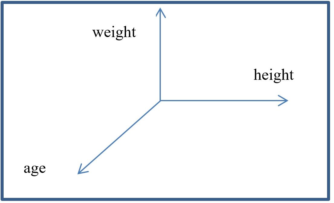
The vector space model refers to a space that can be created to represent samples. A set of axes is created from 0 to some range. Then, any samples can be represented in this space. For example, say that you want to represent 100 people in a room by their age, height and weight. Then, in this case we can create a vector space of 3 dimensions ($ R^3 $) which are age, height, and weight. Now, every person in the room can be mapped to this space based on their values for these 3 parameters.

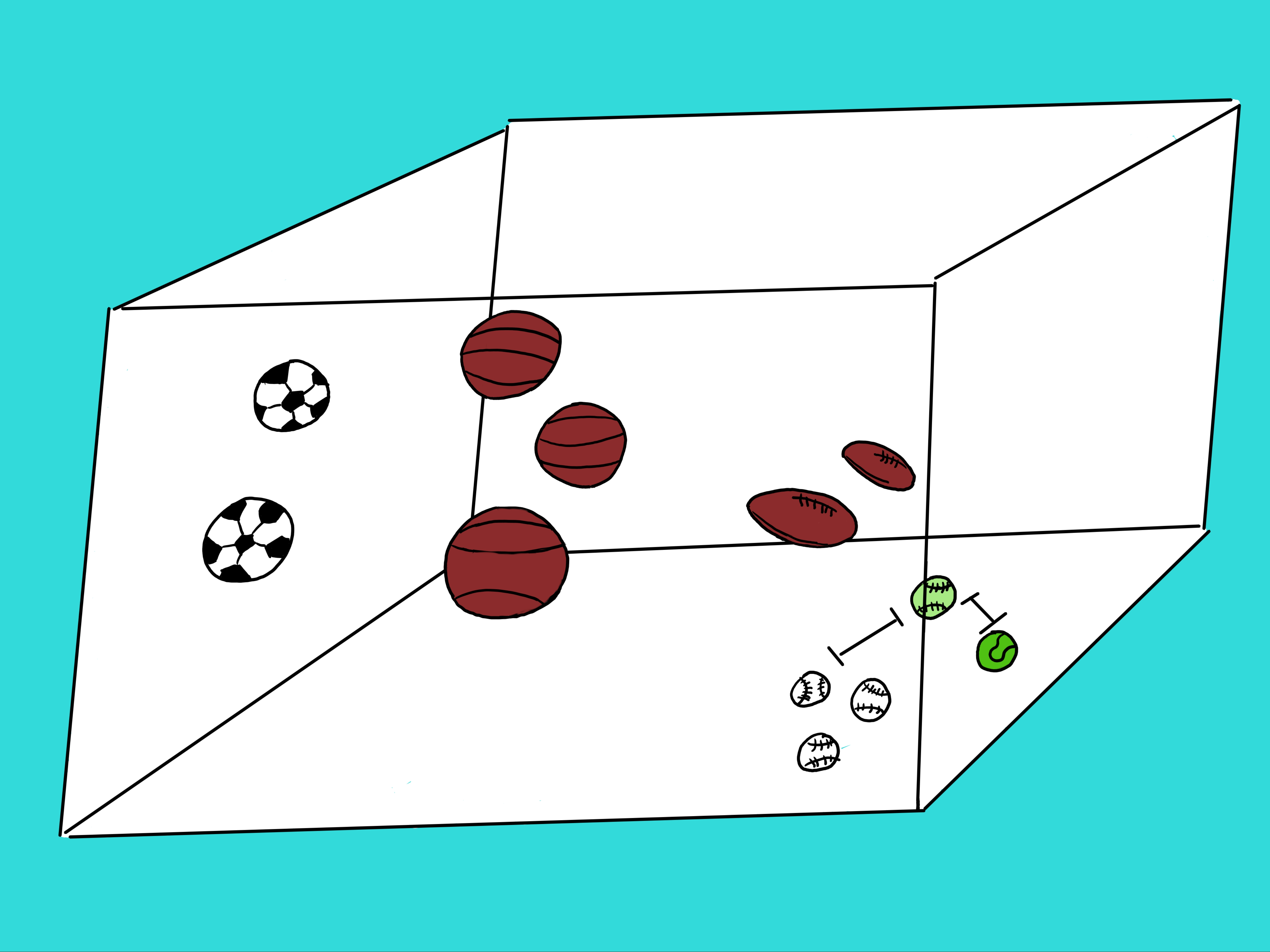
Think of each feature as an axis in this space. If we view the space of balls in the figure below, we immediately know what the ball is. But since AIs do not have eyes (yet), they have to rely on other methods. In this case, KNN should solve this problem. Look at the figure again. In the lower right hand corner there are 3 white baseball balls and one green tennis ball. And then there is an odd looking ball with the shape of a baseball and the color of a tennis ball. What is it? Is this odd looking ball closer to the green tennis ball or the baseball shaped balls? The vector space creates a geometric space where distances can be calculated. Basically, an algorithm like KNN will take a sample in question, say the green baseball, and measure the distance between it and all other balls in this space (i.e. the soccer balls, basket balls, football balls, tennis balls, and baseballs). Once KNN calculates all the distances, it will rank then from lowest to highest distance. Out of these ranked distances, it will select the top \textbf{k} distances and assign to the ball in question the majority class from the set containing just the top \textbf{k} shortest distances. For the given example, if we selected a k=5 then the 5 closest balls to the ball in question (green baseball) would be 3 baseballs, 1 tennis ball, and one football. Since the majority is baseball, KNN would assign the class baseball to our ball in question. From the figure, that would seem like the right answer.

Latent Semantic Analysis (LSA)

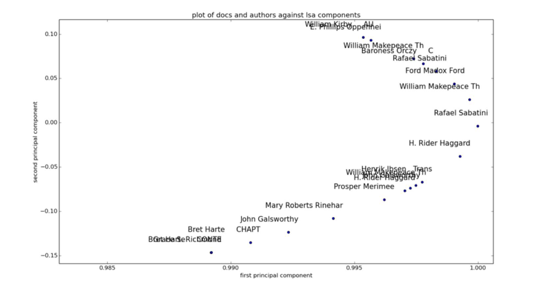
Latent Semantic Analysis (LSA) is a method for discovering relationships or concepts between a set of rows and columns in a dataset such as between documents and terms or between users and movies. These newly discovered concepts can be represented as vectors and they can become a new way of mapping the elements (e.g. the terms). This technique has been used extensively in natural language processing. The concept vectors are discovered using a technique called singular value decomposition (SVD). A very good discussion of SVD can be found in the book: Data-Driven Modeling \& Scientific Computation by J. Nathan Kutz (\babelEN{\cite{kutzRef}}). Once this new space has been created based on the discovered vectors, the elements or terms can be represented in this space. Within this space, distance function metrics can be used to measure similarity between the elements (such as the documents). The following example shows how LSA can be used to plot and capture the relationship between authors of classical literary books. Since this LSA space has considered writing style, it is expected that books by the same author will appear close to each other.

The code to perform the LSA analysis using the SKlearn kit can be seen in the following code segments. It is assumed that you receive a list of text documents or paragraphs in the python list

list_of_texts = [] model = lsa.fit(tfidfMatrix) Similarity = np.asarray(np.asmatrix(dtm_lsa) * np.asmatrix(dtm_lsa_test_sample).T )

The list of texts is vectorized and a tf-idf (term frequency-inverse document frequency) matrix is calculated. From this matrix, an LSA model is calculated. Then, the data is normalized and a similarity metric is calculated between all the elements in the matrix. This similarity metric can help to determine which documents are close to each other. The last part of the code is to print the results using the pandas library. The full code can be seen here:

vectorizer = CountVectorizer(min_df=1, stop_words='english') vec = vectorizer.fit(list_of_texts) dtm = vec.transform(list_of_texts) tfidf = TfidfTransformer() tfidfMatrix_metric = tfidf.fit(dtm) tfidfMatrix = tfidfMatrix_metric.transform(dtm) #lsa = TruncatedSVD(2, algorithm='arpack') ## 2 components lsa = TruncatedSVD(40, algorithm='arpack') ## 40 components model = lsa.fit(tfidfMatrix) dtm_lsa = model.transform(tfidfMatrix) Norm_obj = Normalizer(copy=False).fit(dtm_lsa) dtm_lsa = Norm_obj.transform(dtm_lsa) similarity = np.asarray(np.asmatrix(dtm_lsa) * np.asmatrix(dtm_lsa_test_sample).T ) #print similarity print( pd.DataFrame( similarity, index=list_of_authors, columns=authors_to_compare ) )

Word Embeddings and Neural Nets

Word embeddings are another approach like LSA that allow you to place data in a vector space to discover relationships. Specifically, word embeddings look at the co-occurrence of terms in a document. Word embeddings have existed for a while. However, the improvements in deep learning technologies have led to the development of newer techniques for calculating word embeddings. In particular, Mikolov et al. proposed new algorithms to calculate word embeddings. One of the methods he proposed is called word2vec. Although not a deep neural network (it only uses 1 hidden layer), this technique can be efficiently implemented in PyTorch.

The python code for word2vec is available from the book GitHub at https://github.com/rcalix1 and the book website at www.rcalix.com.

The word2vec code seldom needs to be modified, except for a few parameters. and so I will not discuss it here. Instead, I will focus the discussion on a few aspects of word2vec and utilization.

In particular, word2vec has been widely used for natural language processing. It takes a very large document set and produces a vector space where all the words can be mapped. This vector space is based on the co-occurrence of the words. The dimension $ m $ (number of orthogonal axes) in the space is determined by the number of neurons $ m $ in the hidden layer of the neural network used to perform the analysis. There are various implementations of word2vec. The most common one (the skip gram model) uses a 1-layer neural network to calculate the probability of co-occurrence between the words in a vocabulary defined from the input text set.

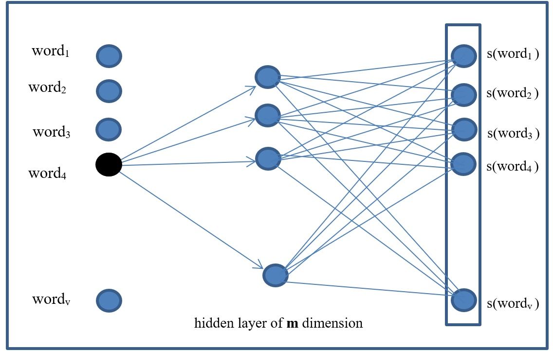
As can be seen in the figure below, the word2vec model has 3 layers:

• input
• hidden 1
• output

The input layer consists of the words in the vocabulary of size “v”. One-hot encoding once again is used here. For example, for the vector [dog, cat, blue] that might represent a vocabulary of a total of 3 words, the word cat would be encoded as follows:

[0, 1, 0]

The vocabulary defines the number of neurons (v) in the input layer. These one-hot encoded vectors for the words in the vocabulary are the inputs to the input layer of the neural network. The outputs of the neural network are also the one-hot encoded word vectors using a softmax function ( s() ).


Similarly to logistic regression, the softmax is used to calculate a probability distribution over the words. In this case, the probability that word $ j $ in the vocabulary co-occurs with the other words in the vocabulary.

Finally, the hidden layer in the model learns the embeddings through the weight matrix (W) for each word. The number of neurons in the hidden layer is selected arbitrarily (m). In this way, each word will have an embedding represented by the $ m $ neurons in the hidden layer. Assuming that the neurons in the hidden layer are called:

$ h_1, h_2, h_3, …,h_m $

Then, an embedding for a word would be as follows:

$ word_j = w_1*h_1+ w_2* h_2 + w_3*h_3 + … + w_m*h_m $

and the weight matrix (W) would look like the following.

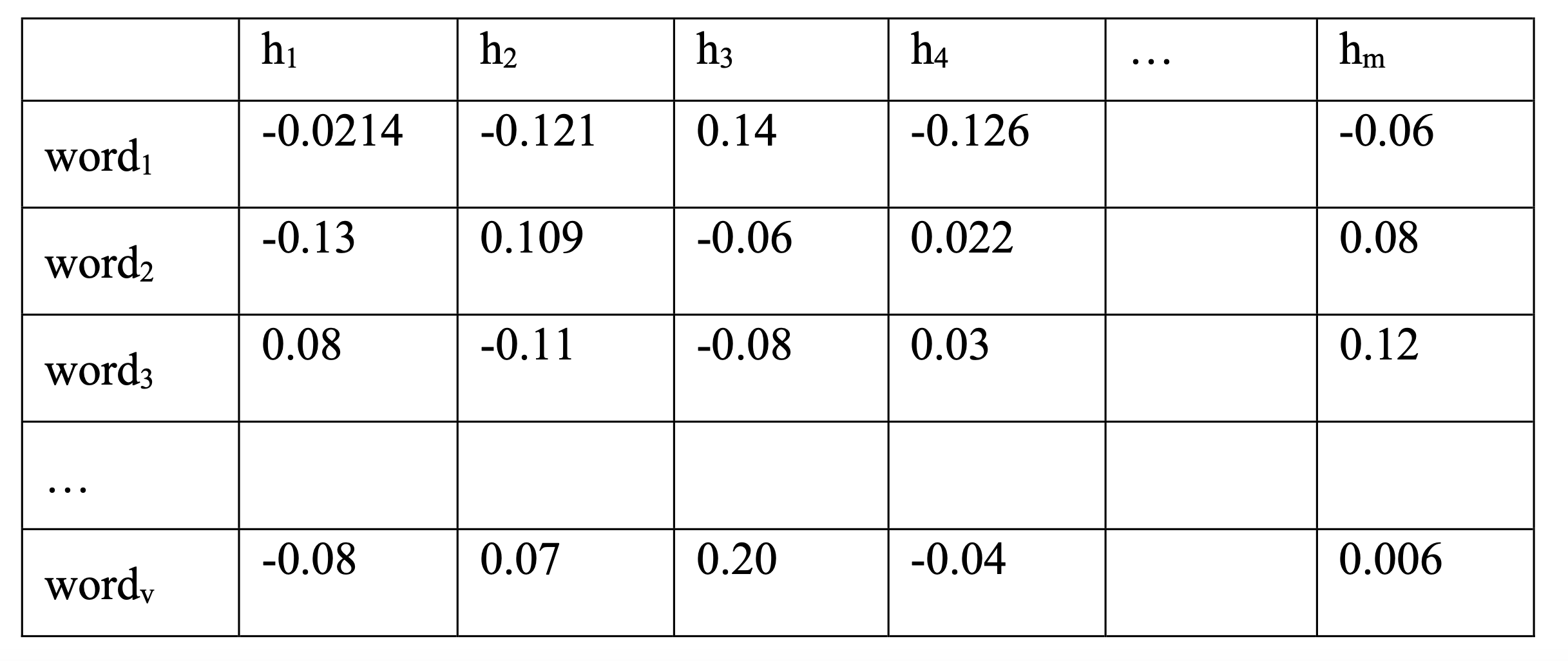
In the next example we can see each word and its vector representation assuming a hidden layer of 6 neurons.

xanax,-0.0214805,-0.121305,0.145779,-0.126096,-0.114934,-0.0642776 sleep,-0.131741,-0.109269,-0.06438,0.0227307,-0.03691,0.0803119 like,0.0839722,-0.111817,-0.0829403,0.0319387,0.129373,0.132047 take,-0.00416363,0.200523,0.029628,0.0190524,-0.130761,-0.00113905 took,-0.0048833,0.0940326,-0.0491561,-0.0484801,-0.0244865,-0.0989419 adderall,-0.0865235,0.0788,0.203447,-0.0491842,-0.00105494,0.00675861 feel,-0.00441388,0.0416924,-0.146706,0.000622775,-0.0609331,-0.0442516 got,-0.120518,-0.0410703,-0.0321787,0.0545667,-0.069366,0.101827

One of the important observations Mikolov et al. made about the word2vec space is that semantic relationships can be discovered by performing vector arithmetic. For instance, given enough data, the following vector arithmetic may be discovered:

king + man – queen = woman

The following code segment shows a simple way of performing vector arithmetic, assuming you have a dictionary of vectors.

dictionaryWordsToVectors = {} f = open("data/ word2vec_vector_space.txt","r") for line in f.readlines(): features = line.split(",") n = len(features) vector = features[1:n-1] vector_float = [float(x) for x in vector] key_word = features[0] dictionaryWordsToVectors[key_word] = vector_float def getVectorFromWord(word): vector = dictionaryWordsToVectors[word] return vector return top_5_closest def findClosestWordToThisVector_list(vector): top_5_closest = [] temp_dict = {} for key, value in dictionaryWordsToVectors.iteritems(): distance_result = distance.euclidean(vector,value) temp_dict[key]=distance_result sorted_x = sorted(temp_dict.items(),key=operator.itemgetter(1)) for i in range(20): top_5_closest.append(sorted_x[i][0]) return top_5_closest a = np.array(getVectorFromWord("prozac")) c = np.array(getVectorFromWord("morphine")) result_vector = a + c result_word = findClosestWordToThisVector_list( a )

Word2vec code

In this section, I will explain some aspects of the word2vec code proposed by Mikolov et. al (2014). I do recommend that you use the available word2vec code from the PyTorch foundation or the one posted on the github repository. That being said, I always wanted to understand word2vec and I am sure you are interested in understanding it as well. Therefore, here I will go over certain parts of the code and try to clarify aspects of it. Generally speaking, I would say that the word2vec code has 2 main components. One component is non deep learning related and the other is the deep learning architecture. Most algorithms we have discussed so far usually are straight forward when it comes to obtaining the data (X) and the labels (y). As such, the focus and challenge has been in the deep learning architecture itself. Given that we have mainly looked at supervised learning algorithms, our data was simple. Feature vectors of images, for instance, and their annotated one-hot encoded labeles. Word2vec is different though. Word2vec is an unsupervised or semi-supervised learning algorithm so there are no annotated labels. Instead, we need to learn mappings (distributed vector representations) from the co-occurrence of things such as terms in a text. This process of getting the initial train data is more difficult. Remember that we said in the previous section that the inputs and outputs of the model are the one-hot encoded words from a large vocabulary. Okay, so here we go. The best way to understand this process of obtaining the $ X $ and $ y $ is with an example. The first thing we need is some libraries and parameters which can be seen in the below code section.

import collections import math import os import random import zipfile import numpy as np from six.moves import urllib from six.moves import xrange import torch vocabulary_size = 55000

Next, let us assume that we have a very very large text like the following named “text8”:

... anarchism originated as a term of abuse first used ...

The first step is is to convert this very large text into a list of words. To achieve this we can use a PyTorch command.

# Read the data into a list of strings f = open("text8") words = torch.compat.as_str( f.read() ).split() print('Data size', len(words))

Our variable \textbf{words} now contains the text in the form of a list.

words = ["anarchism", "originated", "as", "a", "term", "of", "abuse", "first", "used", ...]

The next step is to perform a frequency count of the terms in the list \textbf{words}. The variable \textbf{“count”} is created and used for this purpose. After the frequency count is performed, count looks like the following:

count = [[unk,-1], (the,78), (of, 67), ...]

As can expected, the most frequent terms are “the”, “of”, etc. The variable "UNK" will be used to count infrequent words. That is, not all words will be used as part of the vocabulary. For example, out of 100,000 words, the 55,000 most frequent words could be selected to form the vocabulary. As a result, the remaining 45,000 infrequent words would not be part of the vocabulary and would be counted as unknown words. The variable vocabulary size must be manually set. The code to perform the count can be seen below.

count = [['UNK', -1]] count.extend(collections.Counter(words).most_common(vocabulary_size - 1))

The next step is to build a dictionary of words and keys. Keys are created in order of most frequent using the current dictionary size. Most frequent terms have lower value keys. For example

dictionary = {'and': 3, 'of': 2, 'the': 1, 'UNK': 0}

The code to create the dictionary is provided below. Notice that it uses the previously created frequency counts to assign the keys in ascending order from most frequent to least frequent.

dictionary = dict() for word, _ in count: dictionary[word] = len(dictionary)

The next step is to create the variable “data”. The code below uses the word, key pairs in the dictionary to create the variable “data”. The variable dictionary (which is a python dictionary data structure) has each word and its corresponding key. The resulting “data” object is a list that contains the keys for the words in the original list “words”. So now data has the same information as words except that instead of containing the actual word (such as cat) it cointains its corresponding key (such as 3) from the dictionary. The objects words and data are 2 parallel lists; one list for the words and one list for the keys. So if words looked like this

words = ["hello", "Cat", "tree", ...]

then data now looks like this

data = [17, 3, 53, ...]

where in dictionary we have

dictionary["Cat"] = 3 dictionary["hello"] = 17 dictionary["tree"] = 53

The code to accomplish this is as follows:

data = list() ## count unknown words. Dictionary has 55k frequent terms unk_count = 0 for word in words: if word in dictionary: index = dictionary[word] else: index = 0 # dictionary['UNK'] unk_count = unk_count + 1 data.append(index)

The “if” statement in the code checks to see if the current word from words is in the dictionary (is frequent) or if it is not (infrequent). If the word is not in the dictionary, the unk\_count is incremented. If the word is in the dictionary, then its corresponding key is extracted and appended to data. Unknown words have an index of zero. Once the loop finishes counting the unknown words, the unknown parameter in the frequency count stored in count is updated with this value as can be seen in the next code section.

count[0][1] = unk_count

The object count is a frequency count of the words. The unknown word UNK, which is the first tuple in count initially has a -1 value. After the unknown words count is complete, \textbf{UNK} will have the total of all the unknown terms. Now that we have created \textbf{words} and \textbf{data}, we can visualize them together with the following code. The loop shows the first 15 values for each object.

for i in range(15): print( words[i], " -> ", data[i] )

The result of the visualization is shown below. It shows word and key pairs in the format word -> key.

anarchism -> 5239 originated -> 3084 as -> 12 a -> 6 term -> 195 of -> 2 abuse -> 3137 first -> 46 used -> 59

The next step is to reverse the dictionary and its order. The dictionary looks like this

dictionary = {'and': 3, 'of': 2, 'the': 1, 'UNK': 0}

and when reversed, the dictionary will look as follows and we will call it Reverse_dictionary

Reverse_dictionary = {0: 'UNK', 1: 'the', 2: 'of', 3: 'and', 4: 'one', 5: 'in', 6: 'a', 7: 'to', 8: 'zero', 9: 'nine', 10: 'two', ...}

The code to achieve this is straight forward.

reverse_dictionary = dict( zip( dictionary.values(), dictionary.keys() ))

For the variable \textbf{reverse_dictionary}, the keys are now in the place of words and words in place of the keys. The order is now ascending from 0, 1, 2, etc. This will help to "look up" words by key and speed up retrieval.
We can print the most common words with the following code:

print('Most common words', count[:5]) print( 'Sample data', data[:10], [ reverse_dictionary[i] for i in data[:10] ] )

Okay, after all of this we are now ready to generate a batch of "x" data, and a batch of labels "y". To do this we will use a function called

generate_batch()

Since we are training a word2vec model we know that "x" is a list of one-hot encoded word vector, and "y" is also a list of one-hot encoded vectors. Intuitively, each sample in "x" should look like this

Cat = [0,0,1,0,…]

And each sample in "y" should look like this

Dog=[0,1,0,0,…]

In fact, our dictionary already created the encoding for all words in the vocabulary. So, if our vocabulary contains 55,000 terms, then the dimensionality of our one hot encoded word vectors is 55,000. If a word such as “house” has key 513 in dictionary, then to encode it we create an all zeros vector of size 55,000 where only the position 513 has a value 1 and the rest are zeros. Using the previously created objects (words, counts, data, dictionary, reverse_dictionary) we can now proceed to generate batches.
The main idea is that we will create pairs of words (\textbf{$w_i$}, \textbf{$y_i$}). We will take a window of size \textbf{window_size} (for instance 3) and we will create the vectors. We want to capture context in our training set (X,y). Therefore, we need a way to record the co-occurrence of words.
For example, in a loop, we iterate through the words in a sentence and create a list of the words.
We want to take an input like this
words = ["anarchism", "originated", "as", "a", "term", "of", "abuse", "first", "used", ...]
and convert it into something like this

[anarchism, originated, as] [Originated, as, a] [as, a, term] [a, term, of] Etc.

We do this by passing a window of size \textbf{k} (in this case of size 3) over each word. We grab the current word, and the \textbf{v} words to its right and left.
From each triplet extracted via the window approach such as

[originated, as, a]

we can obtain pairs of words which become the \textbf{x} and \textbf{y} samples. The word pairs can now look like the following

x -> y as -> originated as -> a

By performing this process we have learned that the word “as” co-occurs with the word “originated” and that the word "as" also co-occurs with the “a”. We can expand the size of the window to capture more context (i.e. more word pairs).
Now we can proceed to one-hot encode the word “as”

$x_i$: as = [0,0,0,0,0,0,0,0,1,0,0,0,0,0,…]

and the word “originated” is also one-hot encoded as follows

$y_i$: originated = [0,0,0,0,0,0,0,0,0,0,0,0,0,1,…]

These 2 vectors can now be used to train the Word2vec model which has a simple 1 hidden layer architecture as can be seen in the following illustration

$x_i$ ------- hidden ------ $y_i$

or

as --------- hidden ------ originated

The previously described process can be performed with the following code contained in the function generate_batch()

data_index = 0 def generate_batch(batch_size, num_skips, skip_window): global data_index assert batch_size % num_skips == 0 assert num_skips <= 2 * skip_window batch = np.ndarray(shape=(batch_size), dtype=np.int32) labels = np.ndarray(shape=(batch_size, 1), dtype=np.int32) span = 2 * skip_window + 1 # [ skip_window target skip_window ] buffer = collections.deque(maxlen=span) for _ in range(span): buffer.append(data[data_index]) data_index = (data_index + 1) % len(data) for i in range(batch_size // num_skips): target = skip_window # target label at center of buffer targets_to_avoid = [skip_window] for j in range(num_skips): while target in targets_to_avoid: target = random.randint(0, span - 1) targets_to_avoid.append(target) batch[i * num_skips + j] = buffer[skip_window] labels[i * num_skips + j, 0] = buffer[target] buffer.append(data[data_index]) data_index = (data_index + 1) % len(data) # Backtrack to avoid skipping words at end of a batch data_index = (data_index + len(data) - span) % len(data) return batch, labels

The variable \textbf{data_index} is very important and is necessary to keep track of the current position in the initial input document. So, if the buffer is centered on the word “term” for the below sentence example

["anarchism", "originated", "as", "a", \textbf{"term"}, "of", "abuse", ...]

then the window buffer will contain the terms \textbf{[a, term, of]} and data\_index is equal to 4. Again, we can use the following code to visualize the results of using generate_batch().

print("generate batch does this") print("given the data like this") print('Sample data', data[:10], [reverse_dictionary[i] for i in data[:10]]) print("it generates pairs of words like this") batch, labels = generate_batch(batch_size=8, num_skips=2, skip_window=1) for i in range(8): print( batch[i], reverse_dictionary[batch[i]], '->', labels[i, 0], reverse_dictionary[labels[i, 0]] ) print("this is the batch") print(batch) print("these are the labels") print(labels)

The output of the previous code looks like this

generate_batch() does this given the data like this ('Sample data', [5239, 3084, 12, 6, 195, 2, 3137, 46, 59, 156], ['anarchism', 'originated', 'as', 'a', 'term', 'of', 'abuse', 'first', 'used', 'against']) it generates pairs of words like this: (3084, 'originated', '->', 12 , 'as' ) (3084, 'originated', '->', 5239, 'anarchism' ) (12 , 'as' , '->', 3084, 'originated') (12 , 'as' , '->', 6 , 'a' ) (6 , 'a' , '->', 195 , 'term' ) (6 , 'a' , '->', 12 , 'as' ) (195 , 'term' , '->', 2 , 'of' ) (195 , 'term' , '->', 6 , 'a' ) Where this is the batch "xs" [3084 3084 12 12 6 6 195 195] And these are the labels "ys" [[ 12] [5239] [3084] [ 6] [ 195] [ 12] [ 2] [ 6]]

So we finally have our \textbf{xs} and \textbf{ys} which we can use in our neural network model.
So "xs" is

[ 3084, 3084, 12, 12, 6, 6, 195, 195 ]

And "ys" is

[[ 12] [5239] [3084] [ 6] [ 195] [ 12] [ 2] [ 6]]

Notice that \textbf{xs} and \textbf{ys} are not currently one-hot encoded. This part can be done using built PyTorch functions. The one-hot encoding part for the word vectors can be done in the inference and loss functions of the network architecture.
Finally, keep in mind that the \textbf{generate\_batch()} function is called from the main loop of your PyTorch code. For example like this:

for step in xrange(num_steps): batch_inputs, batch_labels = generate_batch( batch_size, num_skips, window ) y_pred = model( batch_inputs ) loss = loss_fn( y_pred, batch_labels )

Wow! All of that just to get the data for \textbf{xs} and \textbf{ys}.
Now that we have our data \textbf{X (xs)} and \textbf{y (ys)}, we are ready for define the neural network architecture for Word2vec. Word2vec (skip gram model) requires a set of variables to define the parameters of the algorithm. The variables can be seen in the below code section.

batch_size = 128 embedding_size = 128 # Dimension of the embedding vector skip_window = 1 # words to consider left and right num_skips = 2 valid_size = 16 # Random set of words to evaluate similarity on valid_window = 100 valid_examples = np.random.choice(valid_window,valid_size,replace=False ) num_sampled = 64 # Number of negative examples to sample

Once we have our parameter set and the data, we can proceed to define the architecture for the neural network (NN). For the NN definition we need to create an embedding matrix called \textbf{"embeddings"} of size [vocabulary\_size, embedding\_size]. For this example, it is [ 55000, 128].

The Embedding size is the number of dimensions of our embedding space (in this case 128). We can use a PyTorch embedding "look up" table for this.

The function \textbf{nn.Embedding} is a function that returns vectors of size \textbf{embedding\_size} given the provided input words in train\_inputs (\textbf{x}).

## train_inputs = [3084 3084 12 12 6 6 195 195] class word2vec_Net(nn.Module): def __init__(self, vocab_size, n_embd): super().__init__() self.vocab_size = vocab_size self.n_embd = n_embd self.token_embedding_table = nn.Embedding(vocab_size, n_embd) ## [55k, 128] ## self.emb_act = nn.ReLU() self.linear1 = nn.Linear(n_embd, vocab_size) self.act1 = nn.Softmax(dim=1) self.dropout = nn.Dropout(0.25) def forward(self, x): x = self.token_embedding_table(x) x = self.linear1(x) x = self.act1(x) return y_pred

We can define the loss function using NCE which is a method called Noise Contrastive Estimation or try other loss such as cross entropy. The core functions can be seen in the following code listing.

model = word2vec_net() loss_fn = F.nn.NCE() optimizer = torch.optim.Adam( m.parameters(), lr=learning_rate )

That is it!! This concludes the Word2vec algorithm discussion.

Knowledge Enhanced Vector Spaces

In this section, I will discuss how distributed vector representations can be expanded to include knowledge about the world such as common sense knowledge (\babelEN{\cite{havasiRef}}). This can be referred to as knowledge enhanced vector spaces. In the previous section, we described word2vec. However, as of this writing, there are several distributed vector representation techniques such as Word2vec (Mikolov et al 2013), FastText (\babelEN{\cite{bojanowskiRef}}), and WordRank (\babelEN{\cite{ji2015Ref}}). These distributed vectors can be enhanced with knowledge based vector space representations. While the methods of distributed word embeddings have been extensively used, they still lack an ability to obtain true understanding from text. Some believe that prior knowledge of the words is required and not just their co-occurrence in large unlabeled data sets. Attention mechanisms have significantly improved the process of creating word embeddings. This can be seen in the Transformer models (see future chapters).
Knowledge vector spaces can be added to traditional co-occurrence vector spaces to better represent the text samples. Techniques for combining multiple distributed vector representations have been addressed in works such as (\babelEN{\cite{gartenRef}}). Essentially, Garten et al. (2015) argues that different vector spaces can simply be concatenated to each other. That is, for 2 vector spaces for the word \textbf{“w”}, which are $w_1$ = [a, b, c] and $w_2$ = [d, e], a new vector space can be created as $w_3$ = [a, b, c, d, e]. If the resulting vector space gets too big, dimensionality reduction techniques (such as PCA, SVD, autoencoders) can be used to further compress the data.
One particular problem with word embeddings and natural language processing in general (\babelEN{\cite{ling2017Ref}}) is that a lot of information is missing when performing the analysis whether supervised or unsupervised. We as humans, when reading a sentence, do not just rely on the co-occurrence between words to derive meaning from the text. In fact, the meaning is derived from our previous knowledge of the individual words and their context and how they fit in the world. We know things about things and how they make us feel. Most modern word embeddings approaches lack this knowledge. Ling et al. 2017 argues that prior knowledge is important in natural language processing tasks. Therefore, methodologies to enhance the way text is represented are needed. In particular, representations that aren't just based on co-occurrence (e.g. Word2vec), but that are also based on a knowledge vector space for each word. These knowledge based and co-occurrence based vector spaces will serve as the features used to represent the samples. These features can then be used for unsupervised pattern discovery.
In Ling et al. (2017) the authors propose the learning of word embeddings based on co-occurrence of words and based on the semantic similarity between words in a given knowledge base. They adjust their word embedding models by modifying the cost function of the model. In essence, the cost function now includes 2 optimization objectives instead of just one. The first optimization objective is the one related to the co-occurrence of words (such as in Word2vec). The difference is that now the second objective includes the regularization objective related to the similarity of the words in the knowledge base.
The authors in (\babelEN{\cite{lilu2017Ref}}) propose to create affective word embeddings to enhance words in a vector space. Their approach proposes a vector space for each word consisting of orthogonal axes for valence, arousal, potency, etc. Therefore, each word is represented as vectors of these axes. Their methodology learned the values for each axis using a regression model. First, they built a word embedding model based on co-occurrence metrics. Then, they annotated a seed set of words to indicate their given valence, intensity, or other affect level. Finally, with this annotated data, they trained a regression model that was used to predict the affect axis values for all new words. In this way they learned affective vector spaces.
In a knowledge vector space, each word is represented by a set of features that form the vector space. These features will represent well-known characteristics about each word that can be used when processing text to obtain higher understanding of it. For example, the word “depressed” represents a state of a person. Therefore, this word in a knowledge based vector space could be represented by additional words such as: medical state, mental issue, physical issue, related to feelings, physical entity, etc. The word can then be represented as a feature vector using binary values or real valued numbers in a scale from 0-1. The following is a possible representation of the vector. Constructing the knowledge vector spaces is an important task that, in some cases, will be performed automatically and semi-manually but that may require validation by human annotators.

Depressed = [1, 1, 0, 1, 0, etc.]

The representation of this knowledge is very important and will be useful for feature extraction and representation. It will also be useful for pattern discovery via unsupervised learning methods. A more advanced approach to add knowledge into word embeddings is to use additional optimization criteria in the cost functions of the word embedding models (Ling et al. 2017). For example, at a very high level, the criteria in a word embedding model may be to optimize the probability of predicting a word given a context of words such as:

$ J = armax \quad P(w_t | w_{t-1}, w_{t+1}) $

To add knowledge, the objective function can be extended by adding a regularization parameter that accounts for knowledge such as the distance between the word and other context words in a knowledge base. Based on this, the objective function could be re-written as:

$ J = armax \quad P(w_t | w_{t-1}, w_{t+1}) - u * D_k(w_t , [w_{t-1}, w_{t+1}]) $

where $D_k$ is some knowledge based distance function and \textbf{u} is a cost parameter. There are many different parameters that can be explored to adjust these models. The parameters include: different knowledge bases, different distance metrics ($D_k$), different ways of representing distance in the knowledge bases (e.g. distance between nodes), different optimization functions and costs, and different word embeddings models (Word2vec, FastText, WordRank, etc.).

Deep Gramulator

The deep gramulator approach is a combination of the well proven principles of the gramulator (as previously defined) with the abilities of word embedding techniques such as word2vec. As previously defined, the gramulator is a feature extraction technique used particularly in natural language processing. The main idea is that, for a 2 class problem, you want to extract features (e.g. words) that are very frequent in 1 class but infrequent in the other. This helps to better discriminate between the classes. The downside of this approach, however, is that it needs a lot of annotated or labeled data to extract the grams or words from each class that are infrequent in the opposite class. Assuming that the grams are representative of the entire population; then, it can be expected that a classifier will have good performance in the classification task. So the problem is how to get these optimal sets of grams when we do not have that much annotated data. Here, word embeddings can help. As previously mentioned, word embeddings can use the co-occurrence of words in a large data set of documents to create a vector space that can represent some aspects of this relationship. Combining these two frameworks, the gramulator and word embeddings, we can naturally develop the deep gramulator which can be used to find grams from large amounts of un-labeled data by using a small set of annotated text. The algorithm creates the vector space with both text sets (labeled and un-labeled) and then proceeds to find the closest grams from un-labeled texts to the grams of labeled texts. In this case, from a set of originally labeled grams, an expanded set can be obtained. For example, given a 2 class problem, we can use a small set of grams that are very frequent in class 1 but infrequent in class 2, to find more terms in the unlabeled data that might be related to class 1. As a result, you can obtain an expanded set of grams.

Summary

In this chapter, the topic of semantic vector spaces was presented as well as its relationship to neural networks and PyTorch. The vector space model was first introduced to provide the basic framework for other vector spaces based approaches. After discussing the vector space model, a traditional semantic vector space technique called latent semantic analysis (LSA) was also presented. After this, a classic framework called word2vec was discussed. This framework although not a true deep neural network represents an example of the new generation of techniques that have been made available with the advances in deep learning theory and deep learning frameworks like PyTorch. Finally, the chapter presented an example (using the deep gramulator) of how deep learning based techniques and tools can help to automatically obtain features from text for problems related to natural language processing.