Chapter 4 - Getting Started with Deep Learning

Copyright and License

Copyright © by Ricardo A. Calix.
All rights reserved. No part of this work may be reproduced or transmitted in any form or by any means, without written permission of the copyright owner.
MIT License.

FTC and Amazon Disclaimer

This post/page/article includes Amazon Affiliate links to products. This site receives income if you purchase through these links. This income helps support content such as this one.

Deep Learning: Starting at the beginning

In this chapter, I will introduce the topic of deep learning. My goal here is to help students and practitioners alike to get started with deep learning. In particular, I want them to be able to get data and pre-process it for deep learning, load it on their programs, perform classification tasks, and evaluate their results. I will discuss some aspects of the theory providing as much intuition as possible. For this task, I will use Linux, Python, Sklearn, and the PyTorch framework. I will also discuss some aspects of using GPU based hardware by the end of the book. For most of my sample code, I used the conda environment. I installed the PyTorch framework following the instructions in the main PyTorch website (https://www.PyTorch.org/ ).

Things to know about the code

As in the previous section with sklearn, I have included the libraries first. Notice, that I use as many sklearn libraries as possible and only use the PyTorch module when absolutely necessary. The goal, again, is to help the reader to best capture the PyTorch concepts by simplification. Once your skills improve with deep learning frameworks, you will be able to more easily replace sklearn modules with alternative PyTorch modules.

import torch import numpy as np from numpy import genfromtxt from sklearn import datasets from sklearn.datasets import fetch_mldata from sklearn.cross_validation import train_test_split import sklearn from sklearn.preprocessing import StandardScaler from sklearn.metrics import accuracy_score from sklearn.metrics import confusion_matrix from sklearn.metrics import precision_score from sklearn.metrics import recall_score, f1_score import pandas as pd import matplotlib.pyplot as plt

In the previous code section, it can be seen that for our deep learning code to work, we only need a few new libraries. The most important new library is Torch. This of course is the main source of our new code. We will still rely on numpy to efficiently get the data although we can also get data with the statement sklearn.datasets import fetch_mldata. The next important issue in our code to do would be to set some parameters. Deep learning algorithms are iterative in the sense that they load samples in batches to avoid running out of memory. This is very important as it allows you to load millions of data samples in subsets called batches. Therefore, we can set up the parameters for batch processing. In the code below, we can see that we want to load batches of 100 samples each. For a training set of 1,000 samples, we would divide the set into 10 bins of 100 samples each and therefore run 10 batches. Two additional parameters in this code are the learning_rate and the n_epochs. The n_epochs parameter represents the number of times that we will run our main “for” loop. This is the loop that we will run to provide data to our algorithms for training and testing. At this point, an optimization begins to occur which helps the supervised learning algorithm to learn from the samples. The learning_rate value (in this case 0.01) is a very important parameter in the learning algorithm. Simply speaking, it represents the step that is taken in a gradient descent algorithm to find an optimal solution. Think of this like a giant walking over a mountainous region with many peaks and valleys. He is trying to find an optimal location; if the step is too big, the giant could go from peak to peak and skip a valley altogether. On the other hand, if the step is to small the giant may take too long to move in or out of a valley. In terms of PyTorch, the learning rate can affect convergence.
Convergence is the term that means that the iterative algorithm is starting to tend to the optimal solution. The learning_rate can also be assigned a function instead of just a value. This helps to adjust the learning rate in real time while the algorithm is running. Some researchers have suggested that this type of optimization can provide better results than just using a fixed value learning rate.

learning_rate = 0.01 n_epochs = 27000 #1000 batch_size = 100

Deep learning algorithms in PyTorch consist of a basic structure. Simply put, they have:

• Creating the dataset or DataLoaders
• Defining the NN architectures (Inference Function)
• Defining the loss function and optimizer
• Training the model and adjusting the weights

In the next section I will proceed to further elaborate on this. The figure below presents the accuracy plot per epoch of a deep neural net as it is being trained. The x axis represents the epochs over time and the y axis represents the accuracy score. As can be seen, the accuracy is low at first but it starts to improve after a certain number of epochs when the classifier begins to learn and converge.

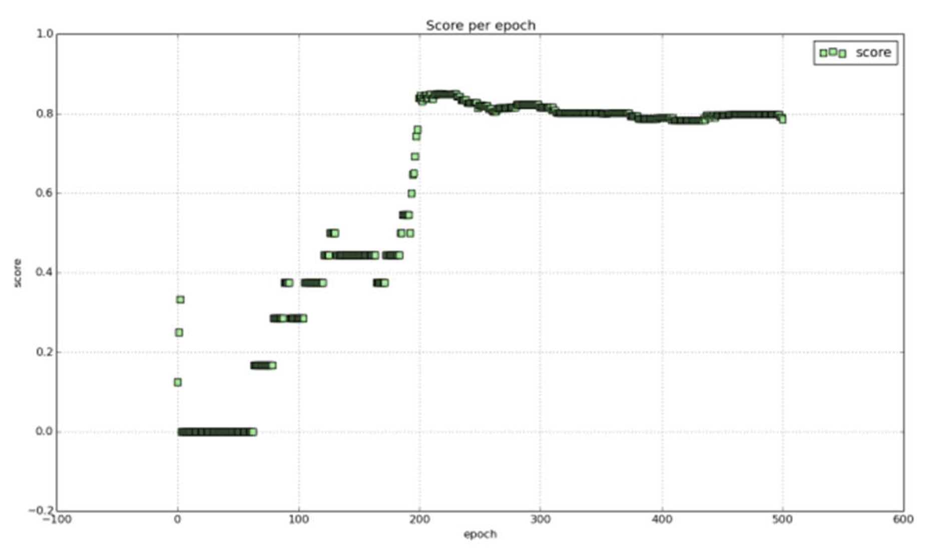
In this example on the figure, a deep net takes a few epochs to learn how to detect and classify the samples. After about 200 epochs, a deep net of say 2 hidden layers stabilizes and is able to maintain a consistent accuracy score.

Getting Started with Deep Leaning

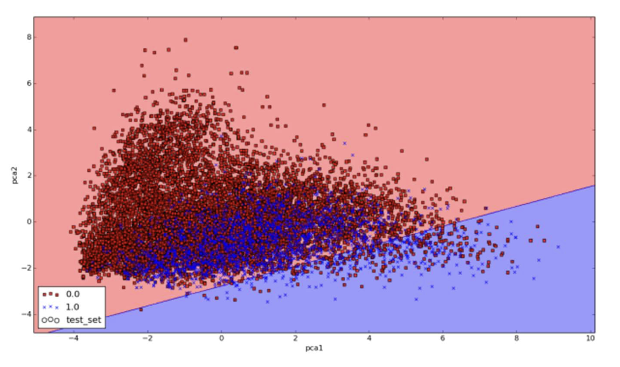
So what’s it all about? Again, my focus here is not to discuss deep learning from the equations point of view or talk about the derivatives. Those are all very important concepts but can be overwhelming when starting. Instead, I want to help the reader write deep learning code with PyTorch. Then, the reader will, no doubt, have many questions where the theory and fundamentals will help him or her to better understand and use the algorithms. The figures below present some of the challenges that must be addressed when dealing with real data. Real data such as language data from Twitter is highly noisy and un-balanced. An imbalance in the data means, for example, that 80% of the samples belong to 1 class and the remaining 20 \% belong to the other class. Therefore, training a classifier to, say, perform emotion classification (where data is highly imbalanced) can be a difficult task. In the figure below, a sample of Twitter data is represented. Each sample in the dataset had multiple features but was compressed into a two dimensional vector for visualization purposes. As can be seen, the data in the figures has a high overlap in the classes and the data is difficult to separate. A linear classifier (the line seen on the graph) can only separate a small portion of the samples and the majority are not easy to separate in this space. The graph below is available on-line in color.

So how can we get more of the samples of one class without getting too many of the samples of the other class? Well, the answer is that we could use another type of line for the separation. For instance, instead of using a straight line we could use a curved line. This is why some algorithms are called linear and others are called non-linear. Non-linear algorithms can sometimes create better separations in the data and therefore obtain fewer errors. In the next Figure, an example of this is shown using Support Vector Machines (SVM). SVM methods can sometimes build better non-linear classifiers because of their ability to project data to higher dimensional spaces. Deep neural networks can be used to learn non-linear models as well. This property of non-linear models can help to obtain better classification accuracy scores. This figure is available on-line in color.

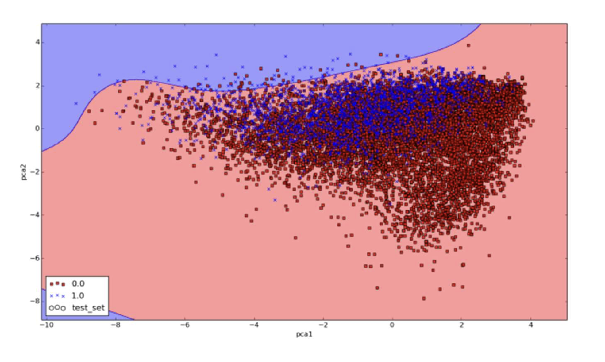
The figure above shows an SVM classifier building a non-linear separation line (the curved line in the graph) on the data. It could be expected that a deep neural network could build even better separation boundaries and that different architectures could give different results. This takes us to the very important aspect of deep architecture. Deep learning architecture is where we define the parameters such as layers and neurons that define a deep neural network. You could think of this as the way that you construct the line that you want to build and use. We will discuss this in the next sections but it is important to know that you can define many deep learning architectures.

Deep Leaning Definition

Deep learning systems are neural networks with many layers. As such, the more layers they have the deeper they are considered to be. In the next sections, I will begin to discuss neural networks. I will focus mostly on intuition when talking about neural networks. I will use linear regression and logistic regression constructs to define them. We can also think of deep neural nets as functions and this will become very useful as we start to program our code. Additional discussions of deep learning theory can be found in many other books such as “Fundamentals of Deep Learning: Designing Next-Generation Machine Intelligence” by Nikhil Buduma and Nicholas Locascio and Deep Learning by Goodfellow et al. (2016).

PyTorch Basics

The main idea with the implementation of deep neural networks in PyTorch is that you need to define a computational graph and run your code through this graph on the CPU (s) or GPU (s).
Here are some of the main aspects of PyTorch to be aware of:

• PyTorch is object oriented
• Tensors are multidimensional arrays
• PyTorch variables are memory buffers that contain these tensors
• We call elements from PyTorch by referencing the object torch as such: torch.nn
• In PyTorch you need to define a graph and then run it

It is now time to write some PyTorch code. Here let us add 2 numbers with PyTorch.

a = torch.tensor( [10] ) b = torch.tensor( [32] ) def model(a, b): return a + b res = model(a, b)

In this code we initialize 2 variables "a" and "b" as torch tensors, and add them together. What is important to note here is that whenever you reference an object in PyTorch with torch, such as initializing the variable "a", you are actually adding elements or nodes to a graph. The graph can be seen in the following figure.

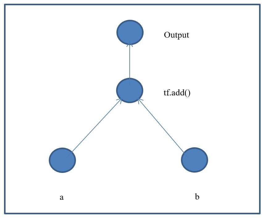
In this case, the command adds the 2 numbers together. The answer for this after printing the results should be 42.

Loading your Data into your PyTorch code

Loading the data can actually be somewhat complicated in PyTorch. One of the issues is that you need to convert the data, say from something like the below example, to another format using one-hot encoding for the labels. This can sometimes be complicated and can cause you problems when writing your algorithms.

class,f1,f2,f3,f4 1.0,6.1,2.8,4.7,1.2 0.0,5.7,3.8,1.7,0.3 2.0,7.7,2.6,6.9,2.3 1.0,6.0,2.9,4.5,1.5 1.0,6.8,2.8,4.8,1.4 0.0,5.4,3.4,1.5,0.4 1.0,5.6,2.9,3.6,1.3 2.0,6.9,3.1,5.1,2.3 1.0,6.2,2.2,4.5,1.5 1.0,5.8,2.7,3.9,1.2

Here, we are looking at the iris data set. The first column represents the annotated class. The IRIS dataset has 3 classes (0, 1, and 2). The other 4 columns represent the features per each sample. The code provided below will show how to read the data. In the code below, we assume that the data is contained in the file iris.csv (available at the book github). We can use the numpy loadtxt() function to obtain the data and to load it into a numpy matrix. Notice that the file has a header for the class and the 4 features. We can easily remove the header by using the parameter skiprows=1 in the numpy.loadtxt() function.

f_numpy = open("data/iris.csv",'r') Matrix_data = numpy.loadtxt(f_numpy, delimiter=",", skiprows=1) #X=Matrix_data[:, [1,2,3,5,6]] X = Matrix_data[:, 1:4] y = Matrix_data[:, 0]

In the previous code we can slice the class column into the "y" variable and the rest of the columns into the "X" variable. Notice that we are following the SKlearn approach from the previous chapters. PyTorch has its own approaches but I have used SKlearn here for the sake of simplicity. When slicing a 2-D matrix ( matrix[i, j] ) we specify the number of rows with \textbf{“i”} and the number of columns with “j”. We can also specify ranges by doing the following: matrix[2:5, :]. The “:” on the “j” index indicates select all columns. If we wanted to select from a list of column indices we could do the following: X=Matrix_data[:, [1,2,3,5,6]].
Now we can split the data.

X_train, X_test, y_train, y_test = train_test_split( X, y, test_size=0.20, random_state=42 )

Similarly to the previous chapters, we can now split the data from "X" and "y" to obtain the train and test sets: X_train, X_test, y_train, y_test. As can be seen in the previous code segment, these data sets are now ready for one-hot encoding. Only the labels need to be one-hot encoded. The code for performing the one hot-encoding step is below. The one-hot encoding function and process was defined in the previous chapter.

y_train_onehot = convertOneHot_data2(y_train) y_test_onehot = convertOneHot_data2(y_test)

In the code above we take the labels in y_train and y_test and pass them through our one-hot encoding function to produce the new variables y_train_onehot and y_test_onehot. You can visualize the new one-hot encoded vectors by running print y_train_onehot[:20,:] for the first 20 samples.
The next step in the process is to scale the "X" data. I suggest running your data with scaling and without to compare the performance of your model. Convergence of your deep learning algorithm and model results can be better with scaled data. In this case we can use SKlearn’s scaling module StandardScaler() to perform this task.

sc = StandardScaler() sc.fit(X_train) X_train_normalized = sc.transform(X_train) X_test_normalized = sc.transform(X_test)

As can be seen in the above code segment, we only need to scale the X data. We can fit a model with the train set and then use that model to scale both the X_train and X_test sets. Now that our data is ready, we want to save some information about the dimensions of the data sets in a couple of variables "A" and "B". This can be very helpful for code re-usability. We will store the number of features in "A" and the number of classes in "B". To obtain these values, we can use the .shape[z] function available to numpy arrays. In the code below we can see an example of how to get this value for "A". In this case, “z” represents the matrix dimension (number 0 for rows ,and number 1 for columns).

# features (A) and classes (B) # A = number of features # B = number of classes # 10 numbers for Mnist (0,1,2,3,4,5,6,7,8,9), # 4 numbers for iris A = X_train_normalized.shape[1] #num features B = y_train_onehot.shape[1] #num classes samples_in_train = X_train_normalized.shape[0] samples_in_test = X_test_normalized.shape[0] print("num features", A) print("num classes", B) print("num samples train", samples_in_train ) print("num samples test", samples_in_test)

At this point, we have completed most of the pre-processing steps and we are ready to define the learning algorithms. This is where we define neural network architecture, the cost functions to be used, and the functions to predict results for given test samples. In the next section, I will implement a linear regression algorithm in PyTorch. After that, I will extend the linear regression framework to build a logistic regression model and later a deep architecture neural network model.

Linear Regression

Linear regression refers to a model for predicting any kind of magnitude (such as housing prices, sales prices, ages, etc.) instead of just classes (e.g. happy vs. sad, etc.). In the next subsections will cover the theory, intuition, and implementation in PyTorch code.

Theory and Intuition of Linear Regression

Two important aspects to consider are the inference equation and the loss function.

• Linear regression inference equation
• Linear regression loss functions

In linear regression, multiple variables and coefficients are combined to form an equation that can be used to fit a particular data set. The fitting process involves an optimization approach that minimizes the Least Squares Error.
The coefficients or weights for each variable are useful in determining the contribution of each variable to the fitted model of the data. The definition of the least squares error function can be seen in the function below (also known as MSE)

$ E = \frac{1}{n} \sum_{i = 0}^{n} (y_i - ( w * x_i + b ))^2 $

Where "n" represents the number of samples.
In linear regression, a line is fitted to the dataset in feature space by minimizing the sum of errors. That is to say, the sum of the error distances between the values in the predicted line and the real values are estimated (see figure below).

In the equation below, the term $ \Biggl \langle \bullet, \bullet \biggr \rangle $ denotes the dot product in the input space between $ w $ and $ x $. Here, $ x $ is the input vector, $ w $ is the weight vector, and $ b $ is the bias.

$ f(x) = \Biggl \langle w, x \biggr \rangle + b $

This simple equation defines the linear regression and the parameters that must be learned given the training data. With this theoretical framework I will now proceed to describe how to code this with PyTorch. The linear regression model is implemented in the code below. The purpose of the code below is to be simple and to show how a linear regression algorithm can be implemented in python using PyTorch.
For our example, we are going to assume a very simple regression problem for housing prices. We are going to have 1 input (1 feature $ x_1 $ ) in our samples (the size of the house) and we will predict 1 output value $ y $ (the cost of the house). Therefore, we will have an equation as such:

$ y = w_1 * x_1 + b $

We will need to solve this equation by learning the values of $ w_1 $ and $ b $ (the parameters) given the training data in $ x_1 $ and $ y $.
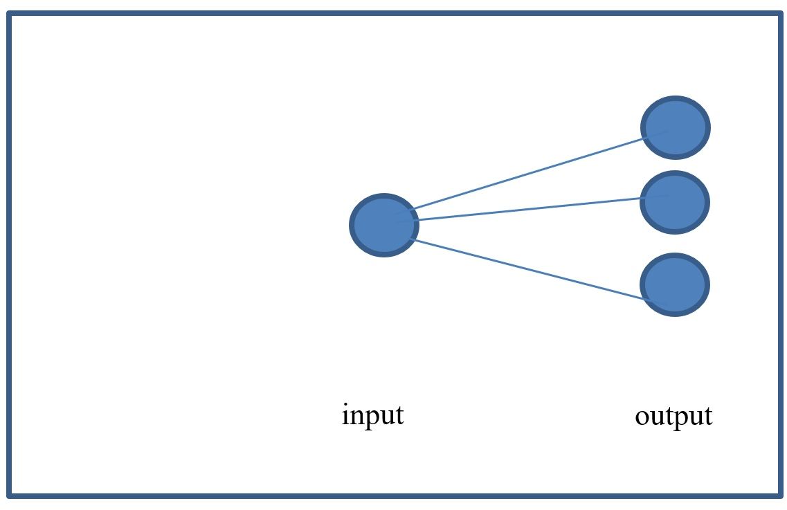
For an equation with 2 input features such as

$ y = w_1 * x_1 + w_2 * x_2 + b $

we can show it in diagram form as can be seen in the figure.

As shown in the previous equation, a linear regression is an equation made up of 3 main elements: x, w, and b. The x value holds the training data (features), w represents the weights per feature, and b is the offset value (bias) learned by the model. These values are directly coded into our algorithm using PyTorch.
The 2 variables, W and b, are variables that define the prediction equation. They are the parameters to be learned. All examples in this book will use these variables whether we are defining logistic regression or deep neural nets. W and b are matrices (tensors) whose dimensions need to be defined. This is where we start to define the architecture of our models. In this case, the dimensions are [1,1] for W and just [1] for b. In the case of W the dimension is [1, 1] because it is for a model with 1 feature ( $ x_1 $) and 1 output value (the predicted housing price y). Think of W as a matrix that connects one layer to the next. In this case, we are connecting the inputs to the outputs.
Okay, so now that we have defined the variables, the next step is to define the equation and define the cost function to learn the parameters (e.g. the weights). To do that, we use the following section of code. This is one of the most important parts of deep learning programming.
In the next section we proceed to train a linear regression model for a wine quality dataset using PyTorch.

Linear Regression model for wine quality data

In this section a linear regression model is trained with PyTorch for a Wine Quality Dataset. Our Wine Quality dataset can also be used in a classification example since the "y" values are discrete and consist of the values [0, 1, 2, 3, 4, 5]. These represent the wine quality rating from 0 to 6.
The data can be used to illustrate the differences between regression and classificatio modeling.
We first add some of our common libraries.

import numpy as np import torch import pandas as pd import sklearn import random import matplotlib.pyplot as plt from mlxtend.plotting import heatmap from sklearn.model_selection import train_test_split from torch.utils.data import TensorDataset, DataLoader from sklearn.metrics import r2_score

The following are the main libraries to define neural network architectures in PyTorch

import torch.nn as nn import torch.nn.functional as F import torch.optim as optim

Next, the parameters are set. These include the learning rate, the number or epochs, and the batch size.

batch_size = 16 learning_rate = 0.0003 N_epochs = 200 ## 1000 epsilon = 0.0001

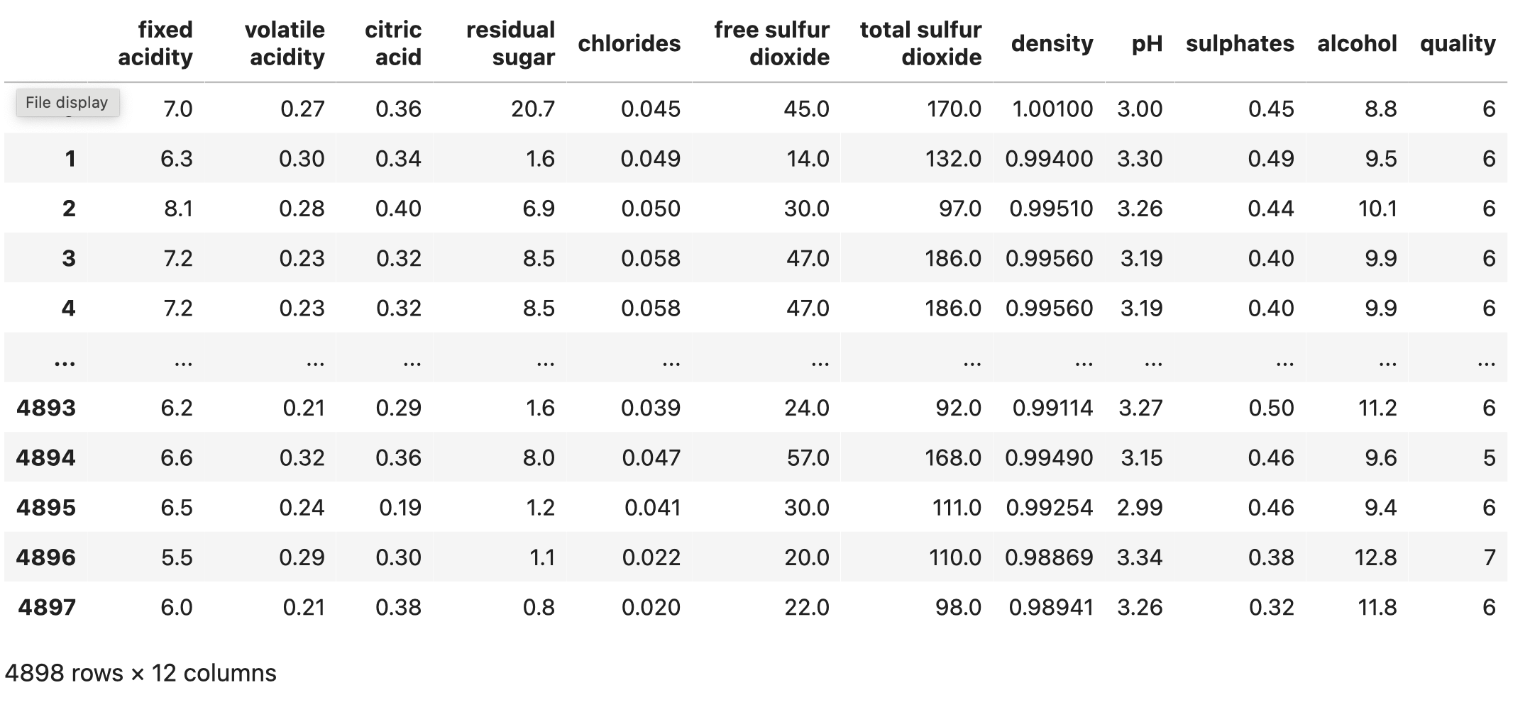
Now we read the data:

path_data = 'winequality-white.csv' WINE_raw_data_df = pd.read_csv(path_data, delimiter=";")

We can print the data with

print( WINE_raw_data_df )

This prints the pandas data frame like so

Now we can print the features in the data frame

headers_list = WINE_raw_data_df.columns.values.tolist() print( headers_list )

which gives us

['fixed acidity', 'volatile acidity', 'citric acid', 'residual sugar', 'chlorides', 'free sulfur dioxide', 'total sulfur dioxide', 'density', 'pH', 'sulphates', 'alcohol', 'quality']

We can also select a subset to focus on

headers_list2 = [ 'density', 'pH', 'sulphates', 'alcohol', 'quality'] print( headers_list2 )

which should give us

['density', 'pH', 'sulphates', 'alcohol', 'quality']

To print a correlation matrix and perform some data science we can run the following

cm = np.corrcoef( WINE_raw_data_df[ headers_list ].values.T ) hm = heatmap(cm, row_names=headers_list, column_names=headers_list, figsize=(20,10))

This gives us the figure as follows

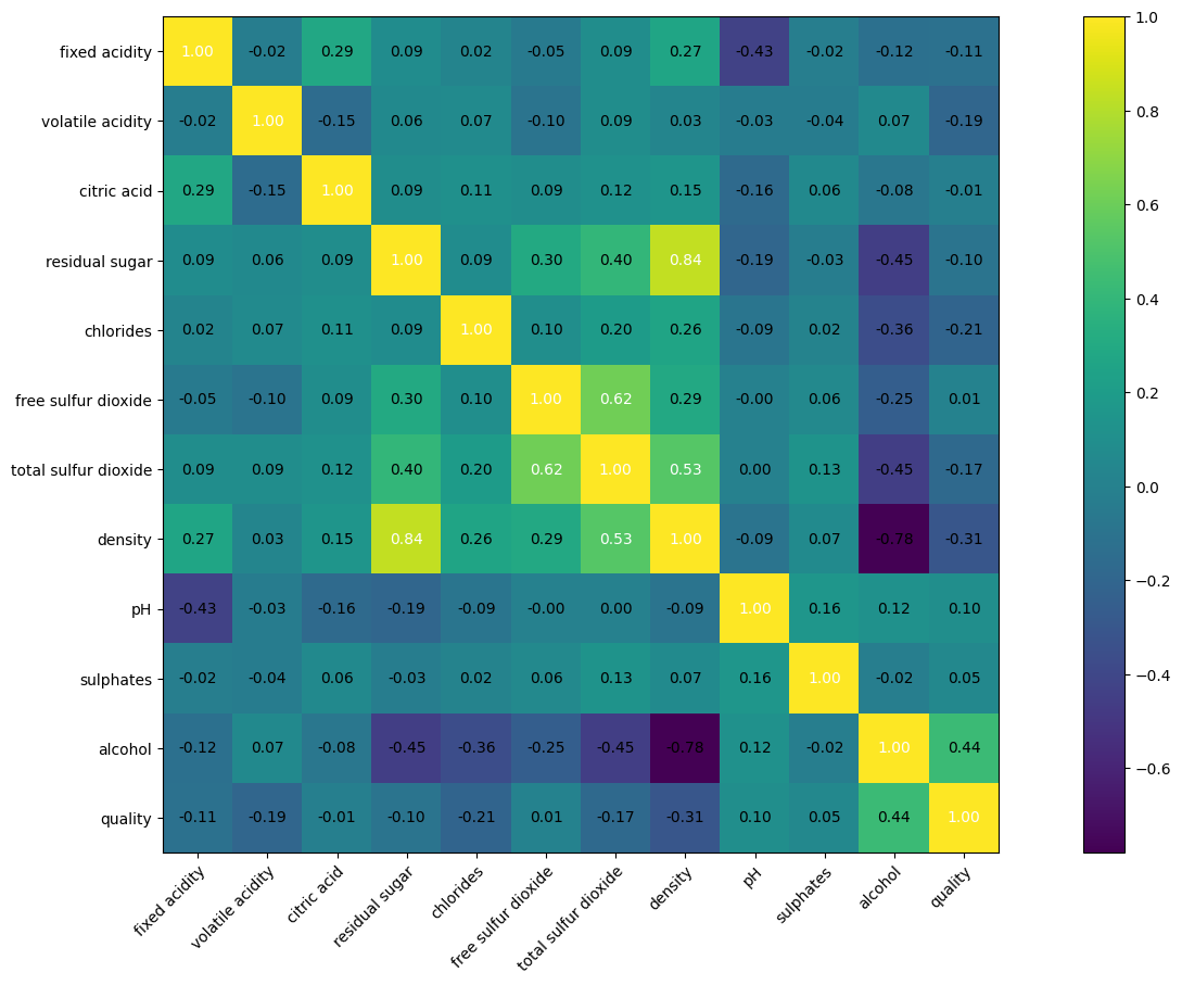
The key is that rows and columns with values very close to zero have no correlation, whereas rows and columns with values close to one (either positive or negative) have strong correlation.
Now we can proceed to process the data and convert from pandas to Numpy.

WINE_raw_data_np = WINE_raw_data_df.to_numpy() print( WINE_raw_data_np )

this will print the numpy array as follows

array([[ 7. , 0.27, 0.36, ..., 0.45, 8.8 , 6. ], [ 6.3 , 0.3 , 0.34, ..., 0.49, 9.5 , 6. ], [ 8.1 , 0.28, 0.4 , ..., 0.44, 10.1 , 6. ], ..., [ 6.5 , 0.24, 0.19, ..., 0.46, 9.4 , 6. ], [ 5.5 , 0.29, 0.3 , ..., 0.38, 12.8 , 7. ], [ 6. , 0.21, 0.38, ..., 0.32, 11.8 , 6. ]])

If we print the shape we can see it is (4898, 12)

print( WINE_raw_data_np.shape )

Now we proceed to slice the wine data into "x" and "y" which gives the dimensions

X = (4898, 11)

y = (4898, 1)

With this we know we have 11 features and one predicted value

X = WINE_raw_data_np[:, :-1] y = WINE_raw_data_np[:, 11:12] print( X.shape ) print( y.shape)

printing the y numpy vector gives us

array([[6.], [6.], [6.], ..., [6.], [7.], [6.]])

I like to split the data randomly every time I train the model. By doing this, I get to see the performance variation. I usually call this a "poor man's ten fold cross validation". I can achieve it quite simply by doing the following:

random_seed = int( random.random() * 100 ) ## 42 X_train, X_test, y_train, y_test = train_test_split(X, y, test_size=0.2, random_state=random_seed) print( X_train.shape) print( X_test.shape) print( y_train.shape) print( y_test.shape)

after the split you can get the following shapes

(3918, 11) (980, 11) (3918, 1) (980, 1)

Sometimes, torch can give you strange errors. One common one relates to the data type being size 64 when it torch wants it to be 32 such as:

dtype('float64')

You can check and change the type like this in numpy array and then change to PyTorch tensors

print( y_test.dtype ) X_train = X_train.astype( np.float32 ) X_test = X_test.astype( np.float32 ) y_train = y_train.astype( np.float32 ) y_test = y_test.astype( np.float32 ) print( y_test.dtype )

after this, the data type should be set to 32.
Now we are ready to convert to PyTorch.

X_train_tr = torch.from_numpy( X_train ) X_test_tr = torch.from_numpy( X_test ) y_train_tr = torch.from_numpy( y_train ) y_test_tr = torch.from_numpy( y_test )

In general, deep learning data likes to be scaled.
There are two main types of scaling which both have worked well for me. Generally speaking, I have used standardization. They are:

• standardization
• normalization

In this example we will standardize by first calculating the data means and standard deviations as can be seen below. The epsilon helps to avoid divide by zero errors.

x_means = X_train_tr.mean(0, keepdim=True) x_deviations = X_train_tr.std( 0, keepdim=True) + epsilon

These can be viewed, for instance, by printing x_means and we get

tensor([[6.8566e+00, 2.7671e-01, 3.3420e-01, 6.3712e+00, 4.5989e-02, 3.5417e+01,1.3811e+02, 9.9402e-01, 3.1890e+00, 4.8992e-01, 1.0511e+01]])

As we saw in the previous chapters, deep learning algorithms are so complex now that using object oriented approaches whenever possible helps to better understand what is going on. In this case we load the data into the torch object "DataLoader" like the code below. the "shuffle" parameter handles randomizing the data as batches are read into the torch model during training.

train_ds = TensorDataset( X_train_tr, y_train_tr ) train_dl = DataLoader( train_ds, batch_size, shuffle=True )

At this stage, we are ready for the linear regression architecture. We define the class for it below. Notice that in the init function we define the number of neurons in the layers. In forward function we then define the neural network sequence from input to output. This even includes the standardization part.

Our architecture object oriented classes will inherit the "nn.Module" class from torch which is a classic example of class inheritance in object oriented programming. We make use of super init function to instantiate the inherited NN class.

The input layer has 11 neurons for the 11 features, and the last layer has 1 neuron for the regression output.

Notice there are no hidden layers or activation functions.

In the following code segment, we define the linear regression architecture.

## Linear Regression class LinRegNet(nn.Module): ## init the class def __init__(self, x_means, x_deviations): super().__init__() self.x_means = x_means self.x_deviations = x_deviations self.linear1 = nn.Linear(11, 1) ## perform inference def forward(self, x): x = (x - self.x_means ) / self.x_deviations y_pred = self.linear1(x) return y_pred

Now, we should be ready to train the model. First we want to define a training function we can re-use. The function has 2 "for" loops. One loop is to repeat the process based on the number of epochs. The second "for" loop is to read the $ xb $ and $ yb $ data in batches from our DataLoader named "train_dl". Here, $ xb $ is run through the model to predict $ y_pred $. The predicted value is compared to the real value in $ yb $ to calculate the loss. This loss is what we minimize according to the definition of the loss function.

def train_loop(N_epochs, model, loss_fn, opt): for epoch in range(N_epochs): for xb, yb in train_dl: y_pred = model(xb) loss = loss_fn(y_pred, yb) opt.zero_grad() loss.backward() opt.step() if epoch % 20 == 0: print( epoch, "loss=", loss)

The following 3 commands from our training function zero out the grads buffer, perform the derivatives to calculate the gradients, and finally take a step to update the weights.

If you noticed, the training function takes arguments for the optimization object and the loss function object. These will be described shortly.

opt.zero_grad() loss.backward() opt.step()

Now we can invoke the core functions and instantiate the "Adam" optimizer and the loss function. Two important items to notice are that the weights from the model are passed to the optimizer with

model.parameters()

and that the loss is initialized to the MSE regression loss function with

loss_fn = F.mse_loss

Now we are ready to call the core functions

model = LinRegNet(x_means, x_deviations) opt = torch.optim.Adam( model.parameters() , lr=learning_rate ) loss_fn = F.mse_loss train_loop( N_epochs, model, loss_fn, opt )

Running the training loop begins the training process and should give us the following output. Notice that the loss is going down. That is the desirable objective.

0 loss= tensor(28.6100, grad_fn=<MseLossBackward0>) 20 loss= tensor(0.3579, grad_fn=<MseLossBackward0>) 40 loss= tensor(0.6686, grad_fn=<MseLossBackward0>) 60 loss= tensor(0.6591, grad_fn=<MseLossBackward0>) 80 loss= tensor(0.4780, grad_fn=<MseLossBackward0>) 100 loss= tensor(0.3440, grad_fn=<MseLossBackward0>) 120 loss= tensor(0.1906, grad_fn=<MseLossBackward0>) 140 loss= tensor(0.6763, grad_fn=<MseLossBackward0>) 160 loss= tensor(0.9073, grad_fn=<MseLossBackward0>) 180 loss= tensor(0.3839, grad_fn=<MseLossBackward0>)

Now we are ready to evaluate our trained model on the test set. Printing the shape of the predicted tensor gives us . The score is measured with the $ R^2 $ also known as the coefficient of determination. This gives us a size of (980, 1) and the metric as follows:

Testing $ R^2 $: 0.3152

The result should be close to 1 to be considered a good result. In future sections we can try better architectures than just linear regression. This is an especially difficult problem to model with regression so the modeling will be challenging but will give us a good dataset to practice on. The code:

y_pred_test = model( X_test_tr ) print( y_pred_test.shape ) print( "Testing R**2: ", r2_score( y_test_tr.numpy(), y_pred_test.detach().numpy() ) )

With the following code we can use the model to predict $ y $ given our $ x $ input vectors of size 11. The predicted torch tensors need to be detached and converted to numpy for further manipulation. This is a common practice when using Torch.

list_preds = [] list_reals = [] for i in range(len(X_test_tr)): print("**********************************") print("pred, real") np_real = y_test_tr[i].detach().numpy() np_pred = y_pred_test[i].detach().numpy() print( (np_pred[0], np_real[0]) ) list_preds.append( np_pred[0] ) list_reals.append( np_real[0] )

The previous code results in the following output.

********************************** pred, real (5.7949276, 6.0) ********************************** pred, real (6.347283, 6.0) ********************************** ... ********************************** pred, real (5.9985185, 5.0) ********************************** pred, real (5.6252785, 6.0) ********************************** pred, real (6.5844297, 7.0)

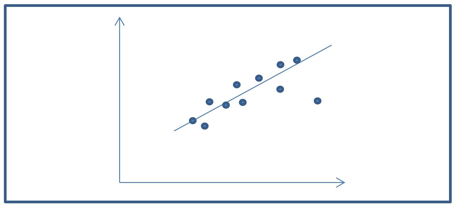
A nice visualization technique to assess our model is to plot together the predicted and real y values from the test set. If perfect, predicted and real values should be in the same point and there should only be one color.

In our graph below we see 2 colors and this shows that the model did not learn so well. The code to do this is as follows:

plt.figure(figsize=(13,4)) plt.plot(list_reals, label='real', color='r') plt.plot(list_preds, label='pred') plt.title("Preds vs. Real") plt.xlabel("Test sample number") plt.ylabel("Rating") plt.legend() plt.savefig("PredVsRealPlot", dpi=300)

and the plot is as follows:

Linear Regression to Logistic Regression and Neural Nets

In this section, we are going to modify and extend our code from the linear regression model so that we can implement logistic regression, one-layer neural nets, and deeper neural networks of multiple layers (Deep Learning). In the following code sections I will make some modifications so that the new models can be implemented easily.

Additionally, we can use the variables "A" and "B" that we previously described to define the number of neurons per layer. In this case "A" represents the number of features in our data set. For example, the iris data set has 4 features per sample ( $x_i = [f_1, f_2, f_3, f_4]$ ). The variable $ x $ is defined as a matrix (tensor) of [None, A] or [None, 4] for this iris dataset. Similarly, $ y $ is defined by [None, B] or [None, 3] where 3 stands for the number of classes which in this case, for the iris dataset, are Setosa, Versicolor, and Virginica.

For the new models, we can continue to use the training function that we previously defined. Although very little changes, it is important to mention that the optimizer and learning rate can be changed and that there are many alternatives that could be used. A lot of research has been done on this topic and it is currently an on-going and open research field. Therefore, many optimization approaches exist and many of them are available in PyTorch.

Regression vs Classification

In linear regression we were training to predict any kind of real valued number. From this point on, we build models that can predict either real valued numbers or discrete classes. The model architectures are similar and we just need to make a few changes usually to output layers and loss functions.

• Predict either real valued numbers (Regression)
• Predict discrete classes (Classification)

For classification modeling, where we predict discrete classes (also called labels), we will usually have the real labels and the predicted labels. Our models will predict the labels and we will need ways of comparing them to the real labels. The following function is a way to evaluate the actual or real classes per sample (y_real) against the predicted classes (y_pred) per sample in a test set. We can compare the two sets of one-hot encoded labels with torch.eq() to measure the accuracy.
The torch.eq() function returns a vector of boolean values that compares the values in two tensors of equal dimensions as can be seen in the following code listing:

y_pred = [1, 2, 3] y_real = [0, 1, 3] torch.eq(x, y) => [False, False, True] or [0, 0, 1]

The loss functions vary for regression and classification. Classification uses Cross Entropy losss (defined later) and Regression uses Mean Squared Error usually (described earlier).

• Classification loss is Cross Entropy
• Regression loss is MSE

Instantiating the different models

So, now we are ready to once again define our model architecture, and define the loss and training functions. This is where the magic will happen and where the code will be specific to the algorithm and architecture being defined. Since this will vary based on model and output type we want to predict, each algorithm will be addressed in its own section later. For now, I will simply define how we can instantiate the architectures. For example, in the next code section I have the core function calls for logistic regression.

model = LogisticRegNet() opt = torch.optim.Adam( model.parameters() , lr=learning_rate ) loss_fn = F.cross_entropy train_loop( N_epochs, model, loss_fn, opt )

If we were defining a deep neural network (with several layers), we can define the function calls as follows (below).

model = DeepLearningNet() opt = torch.optim.Adam( model.parameters() , lr=learning_rate ) loss_fn = F.cross_entropy train_loop( N_epochs, model, loss_fn, opt )

The important aspect is to notice that the structure of the code is mostly maintained and that the only things that change are the architecture definition and the loss function (usually from MSE to Cross entropy).

Reading Data in batches

Earlier in this book, I mentioned that one of the advantages of deep neural networks and PyTorch is that they were designed to process massive amounts of data. Loading millions of records directly into RAM memory would not be suitable for most big data challenges. Instead, to be more efficient we can load data in batches. That is, we can take our data set and divide it into bins of size "N_batch_size".
In the following code section, I will show how to create the batches manually. We need to define the size of each batch (in this case 100 samples) and the size of the train set file. Then we divide number of samples by number of batches. We can then easily slice out the batches from the data by iterating the batch_n index. The dimensions are "sta" for the starting index and "end" for the ending index. In every iteration, we select the rows from "sta" to "end" (sta:end) and all the columns (:).
PyTorch has tools to do this with Torch "TensorDataSet" and Torch "DataLoader" as we previously saw but this is how it works! The code is as follows:

batch_size = 100 num_samples_train_set = X_train_normalized.shape[0] num_batches = int( num_samples_train_set/batch_size ) for i in range(n_epochs): for batch_n in range(num_batches): sta = batch_n * batch_size end = sta + batch_size y_pred = model( X_train[sta:end, :], y_train[sta:end, :] )

What is Number of Epochs?

The previous code section focuses on the training phase in the main loop. This section has 2 nested loops for training. The first one is to train the model for "n_epochs". This allows us to set how many times we want to run the optimization of the model to learn the parameters (i.e. the weight vectors). Stop here and think about this for a second and contemplate what this means. If we set "n_epochs" to 100,000, then it means that the loop will show the same data to the model during training a total of 100,000 times! The data is usually randomized or shuffled each time but still. The model sees the data 100,000 (again and again). Do humans need that many times to learn something? We should think about this.

Logistic Regression

Before we look at the deep neural nets, it is a good idea to look at logistic regression. Logistic regression is still a linear classifier but deep neural nets can build on the ideas of logistic regression. So, basically here we will use all the code we have developed so far. The only main difference is that now we will re-define the code for:

• The architecture classes (Inference class)
• The loss function

The logistic regression inference model class is mainly different from the linear regression approach because we now run our function "nn.linear" which represents the linear equation through a Softmax function.

y = Softmax( torch.matmul(x, W) + b )

Additionally, instead of predicting a real valued number with just one output neuron, we now have several output neurons which represent each possible class (3 in the case of IRIS, or 10 in the case of MNIST or CIFAR-10, etc.). Our Wine Quality dataset can also be used in a classification example since the "y" values are discrete and consist of the values [0, 1, 2, 3, 4, 5]. These represent the wine quality rating from 0 to 6. So, in this case would have 6 classes.

Theory and Intuition of Logistic Regression

Intuitively think of it this way. Imagine you want to predict housing prices given square footage. The value we want to predict is a real value number and not a class. So, this means that you use regression modeling. As such:

$ housing\_price = w_1 * square\_footage + b $

or

$ y = w_1 * x_1 + b $

This formula with values could look like this:

\$250,500 = 50 * 5000 + 500

The model learned the parameters 50 and 500, and with an input of 5000 square feet can predict the housing price. This is a network of one input neuron and one output neuron. One can reason that you can create another similar equation with one input and one output and now you have 2 separate functions with 1 input each that predict one different output each. While these are 2 separate equations, we can combine them together using neural networks so that now both equations work together and can predict 2 outputs given 2 inputs. Basically, that is a model of multiple inputs (two in this case) to multiple outputs (two in this case).

We can extend this idea to models of several classes such as a model for the IRIS data set which has 3 classes, or the wine quality dataset which has 6.

Now, how do we convert real valued numbers such as housing prices to discrete classes such as setosa, virgina, and versicolor?

Well, we know in linear regression we can learn to predict real valued numbers given inputs. From maths we also know that we can run real valued numbers through certain functions to obtain scaled versions of those numbers. In this case a function such as the sigmoid (or the softmax) can do the following:

new_y = S(y)

where

$ y = w * x + b $

This function will take any value and convert it into a value in the range from 0-1. For example:

\$250,500 = 50 * 5000 + 500

new_y = S( \$250,500 )

new_y = 0.80

This allows us to learn functions that predict values between 0 and 1. This is good because these values can also be interpreted as probabilities or strengths of my prediction. As in, I have a 0.80 confidence that the house price is \$250,500. But what if I had 3 possible housing prices: \$150,700, \$250,500, and \$350,400. How can I represent this in the previous equation? Well, if we built one equation for \$250,000. Then we can definitely learn equations for the other 2 prices as such: \$150,700 = 30 * 5000 + 700

\$250,500 = 50 * 5000 + 500

\$350,400 = 70 * 5000 + 400

So now if you notice, we have created a system of 3 equations

$ y_1 = w_1 * x + b_1 $

$ y_2 = w_2 * x + b_2 $

$ y_3 = w_3 * x + b_3 $

If you look at this as a network, we can see that it has 3 output neurons and 1 input neuron and, in fact, the network will look like this:

If we apply our Sigmoid function:

new_y = S(y)

to each equation then we can get a new set of outputs which are now scaled to be from 0..1 like so:

$o_1 = S( y_1 ) = w_1 * x + b_1$

$o_2 = S( y_2 ) = w_2 * x + b_2$

$o_3 = S( y_3 ) = w_3 * x + b_3$

So the formulas, that looked like this

\$150,700 = 30 * 5000 + 700

\$250,500 = 50 * 5000 + 500

\$350,400 = 70 * 5000 + 400

Can now look like this

0.30 = S(30 * 5000 + 700)

0.60 = S(50 * 5000 + 500)

0.70 = S(70 * 5000 + 400)

This intuition hopefully shows you how you can train models to predict confidence values for a specific output neuron such as, confidence that, given a square footage of 5000, the housing price is more likely to be \$250,000 (based on the 0.60 confidence).

For this example we have discretized the housing prices. The model cannot predict values in between these 3 house prices. It can only tell you which one of these 3 is the most likely. To get prices between these 3 we would use Regression. To assign the second housing price when training the model we can use a one hot encoding approach like the following [0, 1, 0] to provide the real values. Notice that if you think of these as probabilities, it means we have 100% confidence that this is for class 2 (second housing price). But our 3 house probabilities do not add up to one (0.30 + 0.6 + 0.7 = 1.6). Having these add up to 1.0 would be desirable. Luckily, we can accomplish this with the Softmax function.

Formally, a Softmax function is a way of mapping a vector of real valued numbers in any range into a vector of real valued numbers in the range of zero to 1 (0-1.0) where all the values add up to 1.0. The result of the Softmax therefore gives a probability distribution over several classes. The softmax function can be written as follows:

$ S(y_i)= \frac{e^{y_i}}{ \sum_{j=1}^{c} e^{y_i} } $

This function takes the y values as inputs (called logit scores), which represent the classes "c", and produces a new y vector where all values add up to 1. An example can be seen here:

[2.0 , 1.0, 0.1] and maps it to => [0.7, 0.2, 0.1]

In python we can test this as follows:

import numpy as np logits = [2.0, 1.0, 0.1 ] exps = [ np.exp(i) for i in logits] sum_of_exps = sum(exps) softmax = [ j/sum_of_exps for j in exps ] print( sum(softmax) )

In the next code segment, the inference function for logistic regression is defined in PyTorch.

y = torch.matmul(x, W) + b y_pred = nn.Softmax( y )

For illustration, the figure below shows the logistic regression neural network for the Iris dataset.

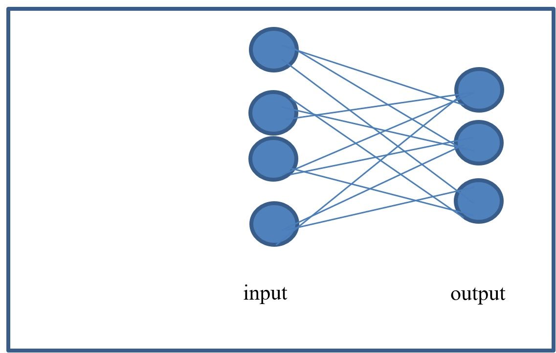
So, assuming we are working with the iris dataset, the features are equal to 4 and the classes are equal to 3. The previous figure shows the architecture for a logistic regression model. If you look closely, you can conclude that a logistic regression model is like a neural network with no hidden layers. There are only 2 layers: the input layer and the output layer. A hidden layer would be a layer in between input and output that connects these 2 layers. The number of neurons in one layer and the number of neuron in the next layer determine the size of the weights matrix W. For the Iris example we can see that W results in a matrix that is [4,3] in size. The b vector (bias) has dimension 3 (for the 3 output neurons). That is, there is now a bias for every neuron in the output layer.

In the linear regression example we used a Least Squares Error loss function (or MSE). In this case we now use a logistic regression cost function. Logistic regression uses a cost function called Cross Entropy. The Cross Entropy compares the real labels to the predicted labels.

There are actually 2 types of Cross Entropy. They are:

• The binary form of cross entropy (for 2 classes)
• The multi-class form

Binary Cross Entropy

The binary form of cross entropy is for cases when you only have 2 classes. The Cross Entropy compares the real labels to the predicted labels using the following equation. The following Cross Entropy loss equation replaces our previously described MSE loss function when optimizing classification models. The Cross Entropy is formally defined as follows:

$ \begin{aligned} cost( g(w^T * x), y ) & = - log( g(w^T * x)) \qquad \longrightarrow if \qquad y = 1 \\ & = - log( 1- g(w^T * x)) \longrightarrow if \qquad y = 0 \end{aligned} $

In the previous cost function definition, g() represents the Sigmoid function. We can also write these equations as follows:

$ \begin{aligned} & - log( h_0(x)) \qquad \longrightarrow if \qquad y = 1 \\ & - log( 1- h_0(x)) \longrightarrow if \qquad y = 0 \end{aligned} $

These 2 equations generate the following graphs:

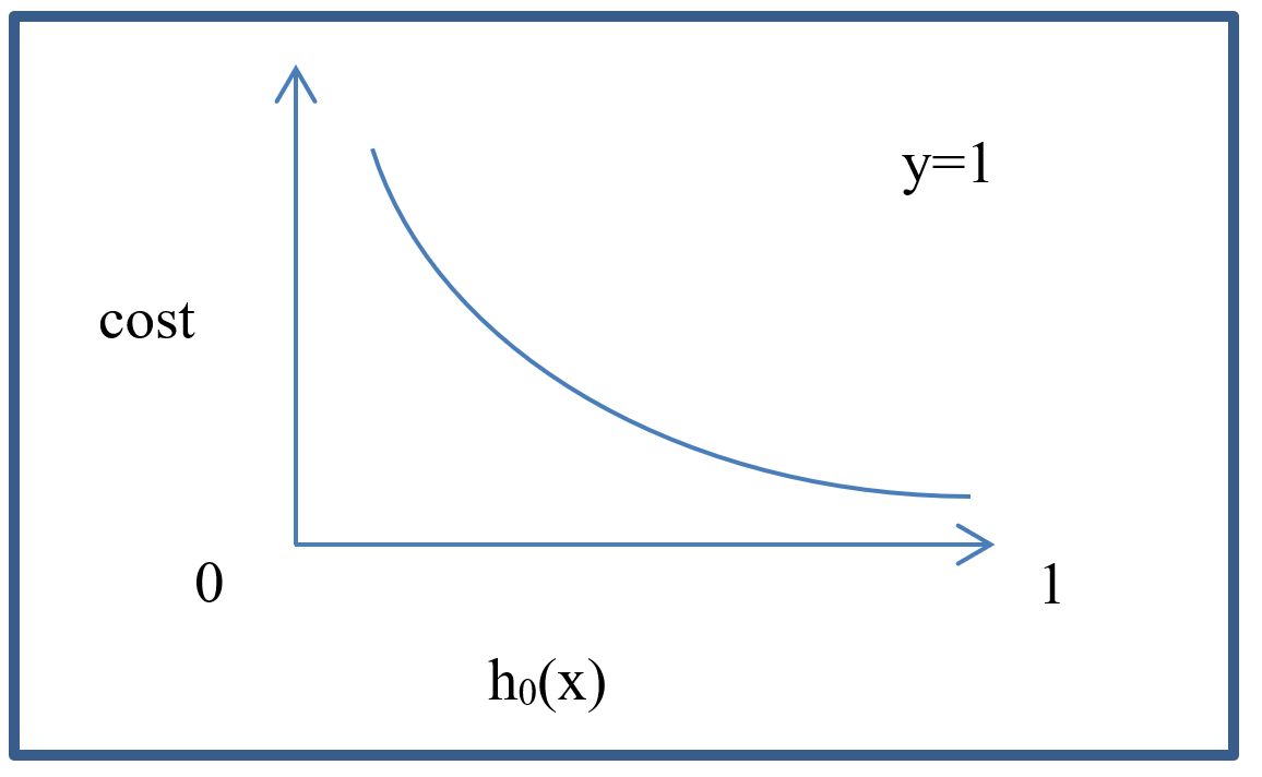
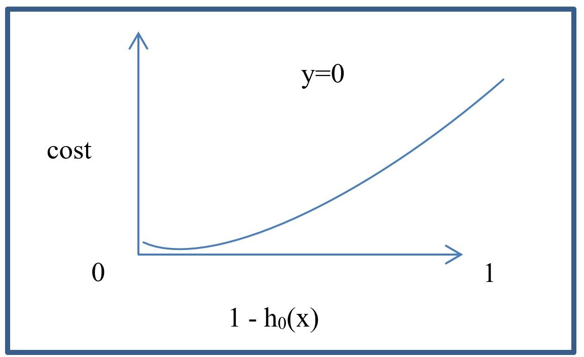
As can be seen in the graphs, the loss has one shape for one class and another shape for the other. For convenience, the previous logistic regression functions can also be written as one function as follows:

$ J( \theta ) = -(\frac{1}{m}) \sum_{i=1}^{m} \quad [y * log(h_{\theta}(x)) + (1-y)* log(1 - h_{\theta}(x))] $

Multi Class Cross Entropy

The following code shows the implementation of the Multi-Class loss function for logistic regression as if we were writing out the equations. One important thing to mention is that I have noticed that this model does not always converge. To correct this, you can use a clipping function like so

y_pred2 = torch.clip_by_value (y_pred, 1e-10, 1.0)

This line of code helps because some values in the process become NaN (Not a Number) and the clipping in the function addresses the problem. This approach of writing out the cost function or equations is not always the most optimal but I have shown it here for contrast between linear regression and logistic regression. A better approach is to use PyTorch built-in cost functions for Cross Entropy calculations. Future code for deep neural networks will abstract this by using the built-in functions.

def loss(y_pred, y_real): y_pred2 = torch.clip_by_value(y_pred, 1e-10, 1.0) dot_product = y_real * torch.log( y_pred2 ) xentropy = -torch.reduce_sum( dot_product, reduction_indices=[1] ) loss = torch.reduce_mean( xentropy ) return loss

The following statement is where we invoke the multi-class cross entropy loss function.

dot_product = y_real * torch.log( y_pred2 )

An easy way to understand the multi-class cross entropy loss function is with an example. Assume we try to classify images of vehicles and we have 5 categories for [plane, car, boat, bike, balloon]. Given a cross entropy model we have the following output vector for this multi-class problem as such:

$ Q_1 = [0.3, 0.2, 0.05, 0.05, 0.40] $

According to this model, the image is 30% plane, 20% car, 5% boat, 5% bike, and 40% ballon. The model is not very confident about what type of vehicle this is. In contrast, the label for each image would tell us with great certainty

$ P_1 = [ 1, 0, 0, 0, 0 ] $

that this is a plane. We can calculate the cross entropy to measure our model's cost.

$ CrossEntropy(P_1, Q_1) = -\sum P_1(i) log Q_1(i) $

If we calculate the values we get:

CrossEntropy = -(1 log 0.3 + 0 log 0.2 + 0 log 0.05 + 0 log 0.05 + 0 log 0.4)

CrossEntropy = - log 0.3

CrossEntropy = 1.20

After training, the model is much better and it can predict the following

$ Q_1 = [0.98, 0.01, 0.01, 0, 0] $

As you can see below, the cross entropy is now lower and optimized.

CrossEntropy = -(1 log 0.98 + 0 log 0.01 + 0 log 0.01 + 0 log 0 + 0 log 0)

CrossEntropy = - log 0.98

CrossEntropy = 0.0202

Therefore, with the cross entropy loss you compare predicted values to the labels. As the prediction improves, the cross entropy value goes down.

Logistic Regression NN Architecture

In this section, I will show the architecture to implement a simple logistic regression NN for the Iris data set and the Wine Data Quality Dataset.

Iris Data set

The architecture for the inference NN is as follows:

class Logistic_Regression_Net(nn.Module): def __init__(self): super().__init__() self.linear1 = nn.Linear(4, 3) self.act1 = nn.Softmax(dim=1) def forward(self, x): x = self.linear1(x) y_pred = self.act1( x ) return y_pred

Notice that the model has 4 neurons in the input layer, and 3 output neurons for the 3 labels. The loss functions can be one of several versions of Cross Entropy such as

loss_fn = nn.CrossEntropyLoss( )

Everything else should be the same as in the Linear Regression code.

Wine Quality Data set

The architecture for the inference NN is as follows:

class Logistic_Regression_Net(nn.Module): def __init__(self): super().__init__() self.linear1 = nn.Linear(11, 6) self.act1 = nn.Softmax(dim=1) def forward(self, x): x = self.linear1(x) y_pred = self.act1( x ) return y_pred

Notice that the model has 11 neurons in the input layer, and 6 output neurons for the 6 labels. The loss functions can be one of several versions of Cross Entropy such as

loss_fn = nn.CrossEntropyLoss( )

Everything else should be the same as in the Linear Regression code.

Now we are ready to add more layers. The next step is to add hidden layers.

Layers of the Neural Network in PyTorch

As we saw in the previous discussions, a logistic regression model is similar to a linear regression model. As you might imagine, a neural network is similar to the logistic regression model. In particular, the neural network now has more layers and the more layers it has, the deeper it becomes.

Layers in between the input and output layers are called hidden layers and help to represent non-linearity along with activation functions.

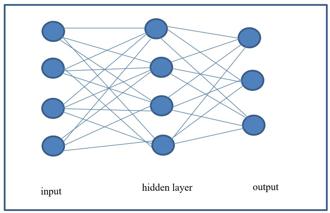
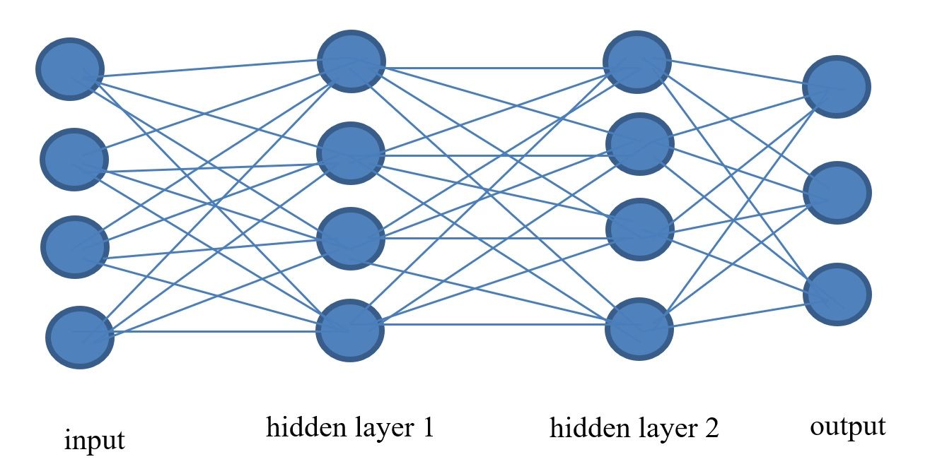
A 1-layer neural network can look like the previous figure and a 2-layer neural network can look like the network in the figure below. As can be seen, we can continue to add layers and this is part of defining the architecture of a deep neural network. In theory, more layers can potentially give a model more power to learn from the data and be better. Notice, however, that this also means that many more parameters need to be estimated (e.g. more weights). Therefore, until recently, this was very expensive to achieve. With the advent of high performance hardware and GPUs, this is now more feasible.

Intuition of adding more layers to a NN

So why can more layers potentially give a model more power to learn and be better? Let us think of an example. In an image processing problem, a neuron in a hidden layer might take as inputs 2 features or input neurons that detect circles. If these two circles are detected by the 2 input neurons, then the neuron in the next hidden layer which is connected to them might infer that a pair of eyes has been discovered. Therefore, this neuron in the hidden layer becomes a face detection or “pair of eyes” detection neuron. Given enough data, the model may discover this intuition and many others.

Going Deep: An N layer Neural Network in PyTorch

We have defined so much of the code already that there really isn’t much left except to define the architecture and cost (or loss) function for the deep neural network. In the next code segments, I will define the 1-hidden layer NN (MLP), and a 2-Hidden layer NN (Deep Learning).
The architecture for an MLP is as follows:

class MLP_Net_Net(nn.Module): def __init__(self): super().__init__() self.linear1 = nn.Linear(11, 8) self.act1 = nn.ReLU() self.linear2 = nn.Linear(8, 6) self.act2 = nn.Softmax(dim=1) def forward(self, x): x = self.linear1( x ) x = self.act1( x ) x = self.linear2( x ) y_pred = self.act2( x ) return y_pred

Notice that the model has 11 neurons in the input layer, 8 neuron in the hidden layer, and 6 output neurons for the 6 labels in the output layer. ReLU activation is used on the hidden layer, and Softmax is used on the output layer. The loss functions can be one of several versions of Cross Entropy such as

loss_fn = nn.CrossEntropyLoss( )

Everything else should be the same

The architecture for the deep neural network is as follows:

class Deep_Neural_Net_Net(nn.Module): def __init__(self): super().__init__() self.linear1 = nn.Linear(11, 15) self.act1 = nn.ReLU() self.linear2 = nn.Linear(15, 8) self.act2 = nn.ReLU() self.linear3 = nn.Linear(8, 6) self.act3 = nn.Softmax(dim=1) def forward(self, x): x = self.linear1( x ) x = self.act1( x ) x = self.linear2( x ) x = self.act2( x ) x = self.linear3( x ) y_pred = self.act3( x ) return y_pred

Notice that the model has 11 neurons in the input layer, 15 neurons in the first hidden layers, 8 neurons in the second hidden layer, and 6 neurons in the last output layer. The loss functions can be one of several versions of Cross Entropy such as

loss_fn = nn.CrossEntropyLoss( )

Everything else should be the same. There are several activation functions but for these 2 architectures I have used the ReLU activation. The ReLU (Hahnloser et al. 2000) function stands for rectified linear unit. It is an optimal neuron for neural networks and it serves as a very effective activation function.

Easy Deep Learning with the Iris dataset

In this section we will train models with the Iris dataset for classification. The Iris data set is a classic dataset that is not too difficult to model for classification.

Let us get started.

First we load the libraries.

import numpy as np import torch import pandas as pd import sklearn import random import torch.nn as nn import torch.nn.functional as F import torch.optim as optim import matplotlib.pyplot as plt from mlxtend.plotting import heatmap from sklearn.model_selection import train_test_split from torch.utils.data import TensorDataset, DataLoader from sklearn.metrics import confusion_matrix from sklearn.metrics import precision_score, recall_score, accuracy_score, f1_score

Now we set the parameters.

batch_size = 16 learning_rate = 0.003 ## 0.001 N_Epochs = 4000 epsilon = 0.0001

Now we can load the data with Pandas

path_data = "iris.csv" iris_raw_data = pd.read_csv( path_data, delimiter=",")

The labels for Iris are strings. We convert them to integers using Pandas as follows:

iris_raw_data.species = iris_raw_data.species.map( {'setosa':0 , 'virginica':1, 'versicolor':2} )

We can view the column headings which gives us

['sepal_length', 'sepal_width', 'petal_length', 'petal_width', 'species']

headers_list = iris_raw_data.columns.values.tolist() headers_list

We can now convert the Pandas data frame to numpy. Printing the shape gives us (150, 5)

## Convert Pandas to Numpy iris_raw_data_np = iris_raw_data.to_numpy() iris_raw_data_np.shape

Now we slice the data for our "X" and "y" data.

X = iris_raw_data_np[:, :-1] y = iris_raw_data_np[:, 4:5]

we can convert the data type to integer

y = y.astype(int)

let us determine the number of labels with np.unique. This give us [0, 1, 2]. There are 3 labels.

the_set = np.unique(y) the_set len( the_set )

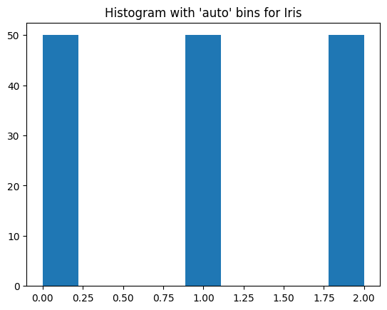
In classification problems, it is a good idea to determine the class balance or imbalance. Imbalanced dataset are more difficult to model. We will see this with the Wine dataset in the next section. Using a histogram can help us to visualize this.

_ = plt.hist(y, bins='auto') plt.title("Histogram with 'auto' bins for Iris") plt.show()

From the histogram below we can see that the classes are balanced.

The shapes can be printed and seen below

print(X.shape) print(y.shape) ## (150, 4) ## (150, 1)

Let us split the data

random_seed = int( random.random() * 100 ) ## 42 X_train, X_test, y_train, y_test = train_test_split(X, y, test_size=0.2, random_state=random_seed) print(X_train.shape) print(X_test.shape) print(y_train.shape) print(y_test.shape) ## (120, 4) ## (30, 4) ## (120, 1) ## (30, 1)

Let us typecast the data to avoid possible errors and then convert to torch tensors.

X_train = X_train.astype( np.float32 ) X_test = X_test.astype( np.float32 ) y_train = y_train.astype( np.int64 ) ## np.long y_test = y_test.astype( np.int64 ) X_train_tr = torch.from_numpy(X_train) X_test_tr = torch.from_numpy(X_test) y_train_tr = torch.from_numpy(y_train) y_test_tr = torch.from_numpy(y_test)

Let us calculate means and standard deviations of the X data for data scaling.

x_means = X_train_tr.mean(0, keepdim=True ) x_deviations = X_train_tr.std( 0, keepdim=True) + epsilon print( x_means.shape ) print( x_deviations.shape ) ## [1, 4] ## [1, 4]

Torch provides a very handy DataLoader that works effieciently with our neural networks.

## X_train.shape[0] -> 120 iris_train_list = [ ( X_train_tr[i], y_train_tr[i].item() ) for i in range( X_train.shape[0] ) ] iris_test_list = [ ( X_test_tr[i], y_test_tr[i].item() ) for i in range( X_test.shape[0] ) ] print( iris_train_list[:3] )

three samples of the data should now look like this

[(tensor([5.1000, 3.5000, 1.4000, 0.2000]), 0), (tensor([6.9000, 3.2000, 5.7000, 2.3000]), 1), (tensor([7.7000, 2.8000, 6.7000, 2.0000]), 1)]

The following command creates the DataLoader

train_dl = torch.utils.data.DataLoader(iris_train_list, batch_size=batch_size, shuffle=True)

we next create the test DataLoader with batch size equal to 30

## X_test.shape[0] -> 30 all_test_data = X_test.shape[0] test_dl = torch.utils.data.DataLoader(iris_test_list, batch_size=all_test_data, shuffle=True)

We know define the architecture for the MLP as follows

## MLP class MLP_Net(nn.Module): ## init the class def __init__(self, x_means, x_deviations): super().__init__() self.x_means = x_means self.x_deviations = x_deviations self.linear1 = nn.Linear(4, 3) self.act1 = nn.Sigmoid() self.linear2 = nn.Linear(3, 3) self.act2 = nn.Softmax(dim=1) self.dropout = nn.Dropout(0.25) ## perform inference def forward(self, x): ## x = (x - self.x_means) / self.x_deviations x = self.linear1(x) x = self.act1(x) ## x = self.dropout(x) x = self.linear2(x) y_pred = self.act2(x) return y_pred

We can try another architecture such as a deep neural network of 2 hidden layers

## Deep Learning with 2 hidden layers class DL_Net(nn.Module): def __init__(self, x_means, x_deviations): super().__init__() self.x_means = x_means self.x_deviations = x_deviations self.linear1 = nn.Linear(4, 15) self.act1 = nn.ReLU() self.linear2 = nn.Linear(15, 9) self.act2 = nn.ReLU() self.linear3 = nn.Linear(9, 3) self.act3 = nn.Softmax(dim=1) self.dropout = nn.Dropout(0.25) ## perform inference def forward(self, x): x = (x - self.x_means) / self.x_deviations x = self.linear1(x) x = self.act1(x) x = self.dropout(x) x = self.linear2(x) x = self.act2(x) x = self.dropout(x) x = self.linear3(x) y_pred = self.act3(x) return y_pred

The next step is to define the train function. We have seen this before.

def training_loop( N_Epochs, model, loss_fn, opt ): for epoch in range(N_Epochs): for xb, yb in train_dl: ## yb = torch.squeeze(yb, dim=1) y_pred = model(xb) ## print( yb.shape ) ## print( y_pred.shape ) loss = loss_fn(y_pred, yb) opt.zero_grad() loss.backward() opt.step() if epoch % 50 == 0: print(epoch, "loss=", loss)

Now we call the Core Functions for the MLP.

model = MLP_Net( x_means, x_deviations ) opt = torch.optim.Adam( model.parameters(), lr=learning_rate ) ## the y_test data can be integers and does not need to be one hot encoded with this function loss_fn = nn.CrossEntropyLoss( ) training_loop( N_Epochs, model, loss_fn, opt )

The torch loss "nn.CrossEntropyLoss( )" is very versatile. It is defined to accept the real labels as integers and does not need them to be onbe hot encoded.

Training gives us the following losses.

0 loss= tensor(1.1073, grad_fn=<NllLossBackward0>) 50 loss= tensor(0.9858, grad_fn=<NllLossBackward0>) 100 loss= tensor(0.7825, grad_fn=<NllLossBackward0>) 150 loss= tensor(0.7099, grad_fn=<NllLossBackward0>) 200 loss= tensor(0.6059, grad_fn=<NllLossBackward0>) 250 loss= tensor(0.6486, grad_fn=<NllLossBackward0>) 300 loss= tensor(0.6819, grad_fn=<NllLossBackward0>) 350 loss= tensor(0.6193, grad_fn=<NllLossBackward0>) ... 3650 loss= tensor(0.5514, grad_fn=<NllLossBackward0>) 3700 loss= tensor(0.5598, grad_fn=<NllLossBackward0>) 3750 loss= tensor(0.5514, grad_fn=<NllLossBackward0>) 3800 loss= tensor(0.5562, grad_fn=<NllLossBackward0>) 3850 loss= tensor(0.5525, grad_fn=<NllLossBackward0>) 3900 loss= tensor(0.5874, grad_fn=<NllLossBackward0>) 3950 loss= tensor(0.5525, grad_fn=<NllLossBackward0>)

We can use our previously defined funtion to determine classification performance.

def print_metrics_function(y_test, y_pred): print('Accuracy: %.2f' % accuracy_score(y_test, y_pred)) confmat = confusion_matrix(y_true=y_test, y_pred=y_pred) print("Confusion Matrix:") print(confmat) print('Precision: %.3f' % precision_score(y_true=y_test, y_pred=y_pred, average='weighted')) print('Recall: %.3f' % recall_score(y_true=y_test, y_pred=y_pred, average='weighted')) print('F1-measure: %.3f' % f1_score(y_true=y_test, y_pred=y_pred, average='weighted'))

Finally, we can estimate the performance metrics for the MLP with Iris

with torch.no_grad(): for x_real, y_real in test_dl: ## batch_size = imgs.shape[0] y_pred = model( x_real ) vals, indeces = torch.max( y_pred, dim=1 ) preds = indeces print_metrics_function(y_real, preds)

the performance can be seen below. Notice that the results are very good.

Accuracy: 0.97 Confusion Matrix: [[ 9 0 0] [ 0 10 1] [ 0 0 10]] Precision: 0.970 Recall: 0.967 F1-measure: 0.967

We can also try the deep learning architecture

model = DL_Net( x_means, x_deviations ) opt = torch.optim.Adam( model.parameters(), lr=learning_rate ) ## the y_test data can be integers and does not need to be one hot encoded with this function loss_fn = nn.CrossEntropyLoss( ) training_loop( N_Epochs, model, loss_fn, opt )

the training gives us the following losses

0 loss= tensor(1.0865, grad_fn=<NllLossBackward0>) 50 loss= tensor(0.5689, grad_fn=<NllLossBackward0>) 100 loss= tensor(0.8691, grad_fn=<NllLossBackward0>) 150 loss= tensor(0.6350, grad_fn=<NllLossBackward0>) 200 loss= tensor(0.5568, grad_fn=<NllLossBackward0>) 250 loss= tensor(0.6729, grad_fn=<NllLossBackward0>) 300 loss= tensor(0.5764, grad_fn=<NllLossBackward0>) 350 loss= tensor(0.5795, grad_fn=<NllLossBackward0>) 400 loss= tensor(0.5524, grad_fn=<NllLossBackward0>) 450 loss= tensor(0.6499, grad_fn=<NllLossBackward0>) ... 3550 loss= tensor(0.5536, grad_fn=<NllLossBackward0>) 3600 loss= tensor(0.6764, grad_fn=<NllLossBackward0>) 3650 loss= tensor(0.5515, grad_fn=<NllLossBackward0>) 3700 loss= tensor(0.5514, grad_fn=<NllLossBackward0>) 3750 loss= tensor(0.5514, grad_fn=<NllLossBackward0>) 3800 loss= tensor(0.5514, grad_fn=<NllLossBackward0>) 3850 loss= tensor(0.5515, grad_fn=<NllLossBackward0>) 3900 loss= tensor(0.5514, grad_fn=<NllLossBackward0>) 3950 loss= tensor(0.5516, grad_fn=<NllLossBackward0>)

finally we predict with the DL model on the test set with

with torch.no_grad(): for x_real, y_real in test_dl: ## batch_size = imgs.shape[0] y_pred = model( x_real ) vals, indeces = torch.max( y_pred, dim=1 ) preds = indeces print_metrics_function(y_real, preds)

The performance metrics can be seen below and they are very good.

Accuracy: 0.97 Confusion Matrix: [[ 9 0 0] [ 0 10 1] [ 0 0 10]] Precision: 0.970 Recall: 0.967 F1-measure: 0.967

That was hopefully easy and a lot of fun. In the next section we explore a more challenging problem. It looks simple, an yet, helps us to see some of the common problems faced when training deep neural networks on noisy or more difficult data.

More Challenging Deep Learning with the Wine Quality dataset

Here we repeat the process from the previous section but on the more challenging Wine Quality data set. We previously used this dataset for regression and now I will use it for classification.

I will only include parts of the code that are new or different from the previous section.

We use the following parameters.

batch_size = 32 learning_rate = 0.001 ## 0.001 N_Epochs = 1000 epsilon = 0.0001

now we read the Wine quality data

path_data = 'winequality-white.csv' WINE_raw_data = pd.read_csv( path_data, delimiter=";" )

we can process the data like we did before

## Convert Pandas to Numpy WINE_raw_data_np = WINE_raw_data.to_numpy() X = WINE_raw_data_np[:, :-1] y = WINE_raw_data_np[:, 11:12] y = y.astype(int)

The wine quality data was designed more for regression modeling. To make our classification modeling more interesting, I am going to process the data so we can also use it for classification. Since the predicted label consists of only 7 rating values, it is possible for us to convert into to classification data.

First we print the labels (ratings) from the y vector with the following

the_set = np.unique(y) the_set len( the_set )

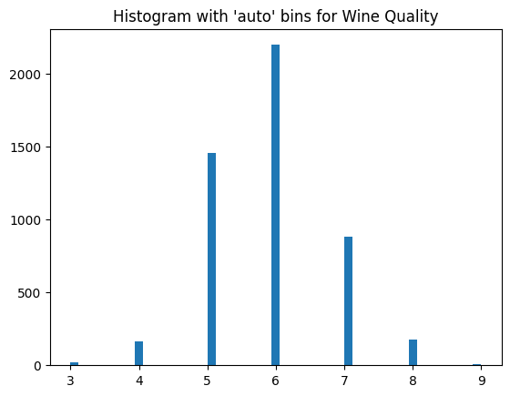
which gives us the ratings [3, 4, 5, 6, 7, 8, 9]. There are 7 ratings and these will become our labels. Let us visualize the label counts with a histogram using the following code

_ = plt.hist(y, bins='auto') plt.title("Histogram with 'auto' bins for Wine Quality") plt.show()

As can be seen in the following histogram, the data is highly imbalanced. This means that this dataset will be more challenging to model for classification.

let us first split the data like in the previous section

random_seed = int( random.random() * 100 ) ## 42 X_train, X_test, y_train, y_test = train_test_split(X, y, test_size=0.2, random_state=random_seed) print(X_train.shape) print(X_test.shape) print(y_train.shape) print(y_test.shape) ## (3918, 11) ## (980, 11) ## (3918, 1) ## (980, 1)

as in the previous section, let us change the data type and conver the numpy arrays to torch tensors.

## fix data type X_train = X_train.astype( np.float32 ) X_test = X_test.astype( np.float32 ) y_train = y_train.astype( np.int64 ) ## np.long y_test = y_test.astype( np.int64 ) X_train_tr = torch.from_numpy(X_train) X_test_tr = torch.from_numpy(X_test) y_train_tr = torch.from_numpy(y_train) y_test_tr = torch.from_numpy(y_test)

we now calculate parameters for standardization

x_means = X_train_tr.mean(0, keepdim=True ) x_deviations = X_train_tr.std( 0, keepdim=True) + epsilon

To create the data loader we first need to create a label map. DataLoader does not allow gaps in label sequences. Our wine quality data does not have labels 2 or 1, for instance. So we need to fix this with a label\_map as follows

## X_train.shape[0] -> 3918 ## label_map = {0:0, 2:1 } ## the_set = array([ 3, 4, 5, 6, 7, 8, 9 ]) label_map = { 3:0, 4:1, 5:2, 6:3, 7:4, 8:5, 9:6 } reverse_label_map = { 0:3, 1:4, 2:5, 3:6, 4:7, 5:8, 6:9 }

with the folowing code we can fix the gap issue and create our list for the data loader as follows

wine_train_list = [ ( X_train_tr[i], label_map[ y_train_tr[i].item() ] ) for i in range( X_train.shape[0] ) ] wine_test_list = [ ( X_test_tr[i], label_map[ y_test_tr[i].item() ] ) for i in range( X_test.shape[0] ) ]

The following 3 examples show us what these lists look like

print( wine_train_list[:3] ) [(tensor([6.3000e+00, 2.8000e-01, 2.9000e-01, 6.8000e+00, 5.1000e-02, 4.0000e+01, 1.4300e+02, 9.9374e-01, 3.4300e+00, 5.9000e-01, 1.1000e+01]), 3), (tensor([7.3000e+00, 2.3000e-01, 3.7000e-01, 1.9000e+00, 4.1000e-02, 5.1000e+01, 1.6500e+02, 9.9080e-01, 3.2600e+00, 4.0000e-01, 1.2200e+01]), 5), (tensor([6.6000e+00, 3.8000e-01, 1.5000e-01, 4.6000e+00, 4.4000e-02, 2.5000e+01, 7.8000e+01, 9.9310e-01, 3.1100e+00, 3.8000e-01, 1.0200e+01]), 3)]

the train data loader is created with the following statement

train_dl = torch.utils.data.DataLoader(wine_train_list, batch_size=batch_size, shuffle=True)

we do something similar for the test data loader

## X_test.shape[0] -> 980 all_test_data = X_test.shape[0] test_dl = torch.utils.data.DataLoader(wine_test_list, batch_size=all_test_data, shuffle=True)

Once the data is ready, we can proceed to define the architectures and train and evalaute our model.

The architecture for the MLP is as follows.

## MLP class MLP_Net(nn.Module): ## init the class def __init__(self, x_means, x_deviations): super().__init__() self.x_means = x_means self.x_deviations = x_deviations self.linear1 = nn.Linear(11, 5) self.act1 = nn.ReLU() ## nn.Sigmoid() self.linear2 = nn.Linear(5, 7) self.act2 = nn.Softmax(dim=1) self.dropout = nn.Dropout(0.25) ## perform inference def forward(self, x): ## x = (x - self.x_means) / self.x_deviations x = self.linear1(x) x = self.act1(x) ## x = self.dropout(x) x = self.linear2(x) y_pred = self.act2(x) return y_pred

and the deep learning architecture can also be defined as follows

## Deep Learning with 2 hidden layers class DL_Net(nn.Module): def __init__(self, x_means, x_deviations): super().__init__() self.x_means = x_means self.x_deviations = x_deviations self.linear1 = nn.Linear(11, 15) self.act1 = nn.ReLU() self.linear2 = nn.Linear(15, 9) self.act2 = nn.ReLU() self.linear3 = nn.Linear(9, 7) self.act3 = nn.Softmax(dim=1) self.dropout = nn.Dropout(0.25) ## perform inference def forward(self, x): x = (x - self.x_means) / self.x_deviations x = self.linear1(x) x = self.act1(x) x = self.dropout(x) x = self.linear2(x) x = self.act2(x) x = self.dropout(x) x = self.linear3(x) y_pred = self.act3(x) return y_pred

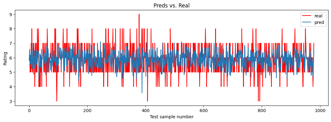
Finally, we proceed to train and evaluate our models. Let us first look at the MLP model

model = MLP_Net( x_means, x_deviations ) opt = torch.optim.Adam( model.parameters(), lr=learning_rate ) ## the y_test data can be integers and does not need to be one hot encoded with this function loss_fn = nn.CrossEntropyLoss( ) training_loop( N_Epochs, model, loss_fn, opt )

the losses for the MLP look as follows

0 loss= tensor(2.0045, grad_fn=<NllLossBackward0>) 50 loss= tensor(1.7409, grad_fn=<NllLossBackward0>) 100 loss= tensor(1.6410, grad_fn=<NllLossBackward0>) 150 loss= tensor(1.4973, grad_fn=<NllLossBackward0>) 200 loss= tensor(1.6076, grad_fn=<NllLossBackward0>) 250 loss= tensor(1.5390, grad_fn=<NllLossBackward0>) 300 loss= tensor(1.5283, grad_fn=<NllLossBackward0>) 350 loss= tensor(1.7964, grad_fn=<NllLossBackward0>) 400 loss= tensor(1.5162, grad_fn=<NllLossBackward0>) 450 loss= tensor(1.6949, grad_fn=<NllLossBackward0>) 500 loss= tensor(1.8356, grad_fn=<NllLossBackward0>) 550 loss= tensor(1.5983, grad_fn=<NllLossBackward0>) 600 loss= tensor(1.6706, grad_fn=<NllLossBackward0>) 650 loss= tensor(1.7059, grad_fn=<NllLossBackward0>) 700 loss= tensor(1.5805, grad_fn=<NllLossBackward0>) 750 loss= tensor(1.6615, grad_fn=<NllLossBackward0>) 800 loss= tensor(1.5225, grad_fn=<NllLossBackward0>) 850 loss= tensor(1.7477, grad_fn=<NllLossBackward0>) 900 loss= tensor(1.6259, grad_fn=<NllLossBackward0>) 950 loss= tensor(1.4791, grad_fn=<NllLossBackward0>)

From the losses, it can be seen that the model has trouble training and learning. Let us verify this by running the model on the test set with the following code

with torch.no_grad(): for x_real, y_real in test_dl: y_pred = model( x_real ) vals, indeces = torch.max( y_pred, dim=1 ) preds = indeces print_metrics_function(y_real, preds)

Running the classification metrics we see that the model does not learn well. It is likely that the class imbalance is affecting performance.

Accuracy: 0.52 Confusion Matrix: [[ 0 0 1 1 0 0] [ 0 3 19 7 0 0] [ 0 3 171 119 0 0] [ 0 3 99 333 0 0] [ 0 0 5 179 0 0] [ 0 0 0 37 0 0]] Precision: 0.402 Recall: 0.517 F1-measure: 0.445

we repeat the exercise with the DL architecture

model = DL_Net( x_means, x_deviations ) opt = torch.optim.Adam( model.parameters(), lr=learning_rate ) ## the y_test data can be integers and does not need to be one hot encoded with this function loss_fn = nn.CrossEntropyLoss( ) training_loop( N_Epochs, model, loss_fn, opt ) with torch.no_grad(): for x_real, y_real in test_dl: ## batch_size = imgs.shape[0] y_pred = model( x_real ) vals, indeces = torch.max( y_pred, dim=1 ) preds = indeces print_metrics_function(y_real, preds)

As can be seen below, the results are not good.

Accuracy: 0.52 Confusion Matrix: [[ 0 0 1 1 0 0] [ 0 0 15 14 0 0] [ 0 0 162 131 0 0] [ 0 0 83 352 0 0] [ 0 0 5 179 0 0] [ 0 0 0 37 0 0]] Precision: 0.401 Recall: 0.524 F1-measure: 0.445

So, that is it. That completes the Wine data discussion for this section. It seems to be a more challenging problem. I encourage the reader to try to improve the results. Consider trying the following:

• Combining classes
• trying different architectures with deeper networks
• over-sampling or under-sampling the data

Summary

In this chapter, the main topic of deep learning was introduced. The chapter addressed the PyTorch environment and code definitions as well as theoretical concepts for deep learning. Issues about neural network architecture and performance evaluation were also presented. Finally, several coding examples using python, Sklearn, numpy, and PyTorch were provided in an incremental fashion for the algorithms of linear regression, logistic regression, 1-layer neural networks (MLP), and n-layer neural networks (Deep Learning). The next chapters will further look at other methods that can be implemented with PyTorch and, in particular, that are more advanced algorithms.