Chapter 6 - Convolutional Neural Networks (CNNs)

In this this chapter, I will focus on a more advanced topic in deep learning called Convolutional Neural Networks (CNNs). This type of technique has been used extensively for image processing. It has the capability to learn the features from the image data without human intervention. The explanations in this chapter assume that you have read previous chapters of this book. I will re-use a lot of the code we previously used to define our logistic regression and deep neural network algorithms. There will be a few new functions to define a convolutional network architecture and to perform some new operations but you will notice how much of the CNN code is similar to what we have done in previous chapters.

Copyright and License

Copyright © by Ricardo A. Calix.
All rights reserved. No part of this work may be reproduced or transmitted in any form or by any means, without written permission of the copyright owner.
MIT License.

FTC and Amazon Disclaimer

This post/page/article includes Amazon Affiliate links to products. This site receives income if you purchase through these links. This income helps support content such as this one.

Convolutional Neural Networks

In this this chapter, I will focus on a more advanced topic in deep learning called Convolutional Neural Networks (CNNs). This type of technique has been used extensively for image processing. It has the capability to learn the features from the image data without human intervention. The explanations in this chapter assume that you have read previous chapters of this book. I will re-use a lot of the code we previously used to define our logistic regression and deep neural network algorithms. There will be a few new functions to define a convolutional network architecture and to perform some new operations but you will notice how much of the CNN code is similar to what we have done in previous chapters.

The Data

CNNs have traditionally been used on image data. The firs data set we will use to learn about CNNs is called the MNIST dataset. It is a well known annotated dataset containing images of hand written digits in the range of 0, 1,..,9. The data set consists of a train set, a validation set, and a test set. It has around 70,000 images of dimension 28x28 in grey scale.

Convolution and CNNs Defined

So, what is a convolution? Convolution is a mathematical operation between two functions \textbf{f} and \textbf{g} to produce a new modified function \textbf{(f * g)}. It is a special kind of operation that involves the multiplication of 2 input functions with some additional conditions. As an example, in image processing this could mean the convolution between function \textbf{g} (an image) with a function \textbf{f} (a filter) to produce a new modified version of the image. Image processing uses filters to identify features in images such as for edge detection. Edge detecting filters, for instance, look for areas in an image of high variation to identify edges. That is, where the values of the pixels are all about the same may be considered a background but where the values are consistent and then start changing may mean that an edge is detected. In the previous chapters, we have multiplied a data set matrix X with a weight matrix W. Applying a filter to an image is a similar process where you multiply (using a convolution operation) an image matrix (equivalent to X) with a filter matrix (similar to the weights). In fact, there are many types of filters that could be defined for image processing. In the past, these filters had to be defined by human feature engineers. The insight given by convolutional neural networks is that, given training data with labels, these filters (the convolution filters) can be learned by the model by learning the weights. And because the neural networks have multiple layers, convolutional filters learned from one layer can be used to transform inputs for the following layer.

Architecture for a Convolutional Neural Network with MNIST

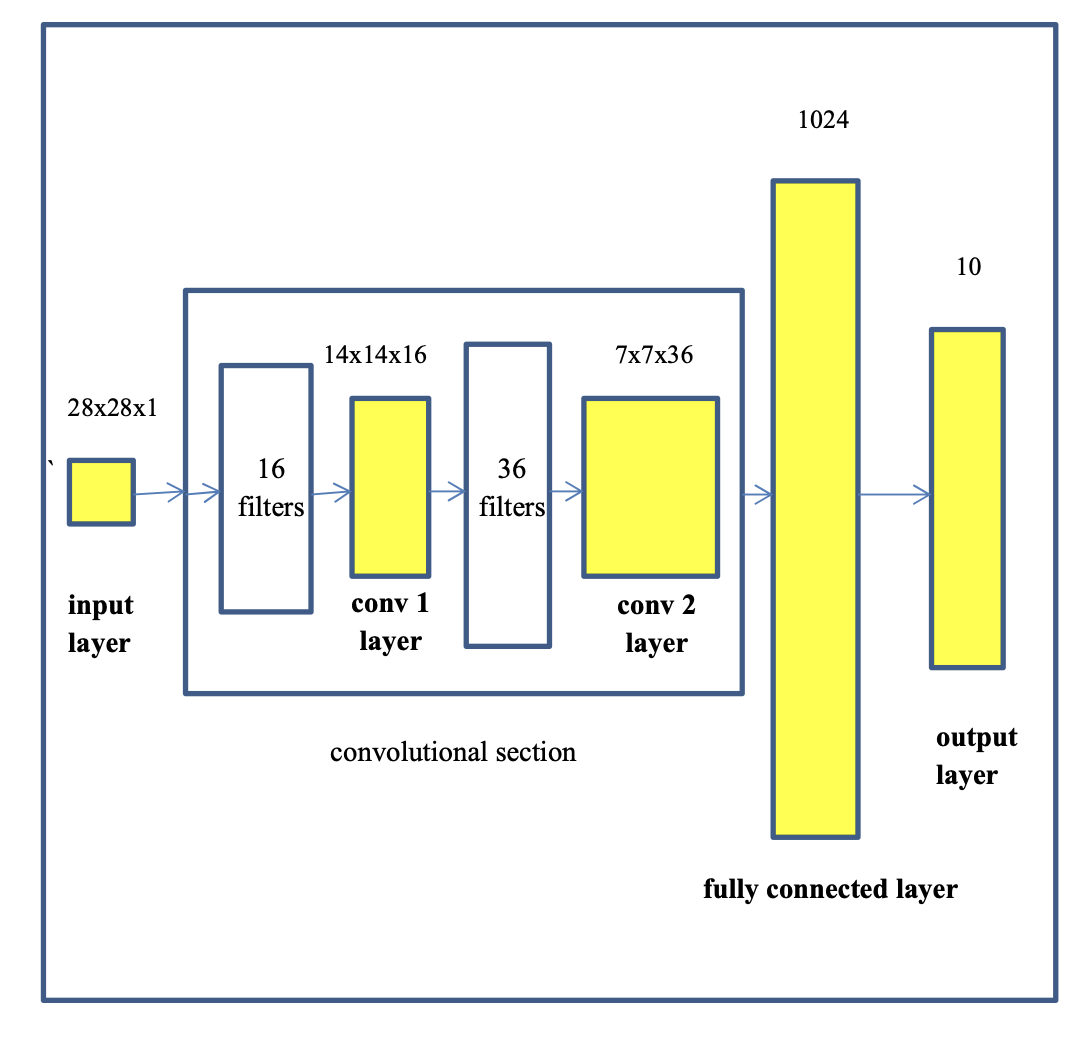
In this section, I will provide the main description of the architecture of the convolutional neural network and show some diagrams to better interpret the intuition of convolutional neural networks (CNNs). The diagram below shows an overview of the model we are going to build to perform image classification of hand written digits. The CNN we are going to use as our example consists of the following layers:

• input layer (the image)
• convolutional layer 1
• convolutional layer 2
• fully connected layer
• output layer

There are many details that could be described to define the architecture of a convolutional neural network. However, implementing one in PyTorch is not that difficult. Defining the architecture of a CNN is similar to how we defined the architecture of our previous deep learning classifiers. We need to define the number of layers and the size of each layer. In our previous layer definitions, the matrix multiplication was our main operation. When implementing a convolutional layer the main operation is a convolution. For convenience, here we will think of convolutional layers as black boxes of filters with inputs and outputs. Therefore, whenever we define a convolutional layer we need to define the following: The number of inputs and the size of each input. In this case, the size of each input refers to the size of the image. In the case of Mnist, the images are 28*28 each. The number of inputs refers to the number of channels for the image. For instance, 1 channel for grey scale images and 3 channels for RGB or color images (color images are actually 3 matrices of size 28*28). The number of filters is a value that is defined by the network architect. For example, 24 filters or 16 filters. These are the convolutional filters which will be applied to the images. In the case of 16 filters, it means that 16 different filters would be applied to 1 input image to produce 16 new processed images (these new 16 processed versions of the input images would be referred to as producing 16 output channels). The size of the filter is also defined (for instance a filter of 5*5). The number of outputs, as indicated in the previous bullet, refers to the output output channels and consist of the processed images after convolution.
It is important to note that the convolution process is a bit more complicated when the number of inputs is more than 1; for example, when a convolutional layer has 16 input channels (16 versions of the input image) to the layer and 36 filters to be applied. In this case each input channel needs to be processed by all 36 filters. In the end, the layer will output 36 processed images. Additionally, it is important to note that the output images may not always retain their original size (e.g. 28*28 for mnist). Instead, after each layer, the processed images may be down sampled. This is called maxpooling. In our example, we will down sample from 28x28 to 14x14 and then to 7x7. So let us discuss the architecture of the CNN we are going to implement. The CNN will have the following characteristics.
1 input layer, 2 convolutional layers, 1 fully connected layer, and 1 output layer
The input layer will consist of images of 28x28 with 1 channel The first convolutional layer will have 16 filters. Each filter will be of size 5x5. The images will be down sampled to 14x14. The second convolutional layer will have 36 filters. The filters will be 5x5. The images will be down sampled to 7x7. The fully connected layer will have 1024 neurons. This is a normal layer that will connect the output of the second convolutional layer to the output layer. The output layer has 10 nodes which represent the 10 classes in the MNIST dataset.

Based on the previous characteristics (see figure above), we can define our network architecture dimensions as follows:

• Input layer: 28x28x1
• Conv layer 1 output: 14x14x16
• Conv layer 2 output: 7x7x36
• Fully connected layer: 1024
• Output layer: 10

The figure above presents a more visual representation of our example convolutional neural network.

Coding a CNN for MNIST

Once we have defined the architecture, we are ready to start coding our CNN. The code in this chapter is very similar to code from previous chapters. Therefore, I will only focus on new aspects of the code and will try not to repeat descriptions that have been provided in previous chapters. We can use the following libraries

import torch import numpy as np import os from torchvision import datasets from torchvision import transforms import matplotlib.pyplot as plt from PIL import Image from sklearn.metrics import confusion_matrix from sklearn.metrics import precision_score, recall_score, accuracy_score, f1_score import torch.optim as optim import torch.nn as nn

The first part of the code that needs to be defined is the section used to set the algorithm parameters.

learning_rate = 0.003 N_Epochs = 20 batch_size = 32

Most of the parameters defined in this section are similar to parameters we have used in previous chapters. A new parameter is the dropout. The dropout is a parameter for a technique first defined by Geoffrey Hinton. Dropout is a technique that helps to perform a better optimization during the weight search. Every iteration during training, the dropout percent of connections (weights) is dropped.
At the heart of a CNN there are 2 main operations which are the convolution and the maxpool operation. The convolution code can be seen below. As can be seen, it takes images and filters and performs a convolution operation. The strides parameter defines how the filter will slide across the image (e.g. every pixel, every 2 pixels, etc.). Therefore, strides can achieve the same objective and maxpooling. For instance, a stride of 2 can be seen as maxpooling the image by a factor of 2 as well. Both approaches in the literature have been found to achieve similar results.

model = nn.Sequential( ## Convolution layer 1 nn.Conv2d(3, 16, kernel_size=5, stride=1), nn.LeakyReLU(0.2), nn.BatchNorm2d(16), nn.MaxPool2d(2, 2), nn.Dropout(0.25), ## Convolution layer2 nn.Conv2d(16, 32, kernel_size=5, stride=1), nn.LeakyReLU(0.2), nn.BatchNorm2d(32), nn.MaxPool2d(2, 2), nn.Dropout(0.25), )

The maxpool or stride operation are used to down sample the images. For instance, in the case of the mnist images which have a size of 28x28, every time the images or their filtered equivalents pass through a maxpool function (or use stride), the result is that the image is reduced in size. During the first convolution (convolution layer 1), the filtered images are down sampled from 28x28 to 14x14. In this MNIST example, I will use maxpool which means I also need to set the strive value to one.
In the previous code listing, the activation is ReLU, and normalization and dropout layers can also be seen.
To keep things simple here, I will read the MNIST from the datasets module in torchvision.

data_path = "data/MNISTdata/" mnist_train = datasets.MNIST(data_path, train=True, download=True) mnist_test = datasets.MNIST(data_path, train=False, download=True)

The datasets module also has a nice way of applying filters to the data so that it can be converted to Torch tensors. Many filter can be applied but here I only use the \textbf{Transforms.ToTensor()} which is necessary to convert the whole dataset to torch tensors.

mnist_train_tr = datasets.MNIST(data_path, train=True, download=False, transform=transforms.Compose([ transforms.ToTensor() ])) mnist_test_tr = datasets.MNIST(data_path, train=False, download=False, transform=transforms.Compose([ transforms.ToTensor() ]))

we can now proceed to display an image with the PIL image module

Image.fromarray( mnist_test_tr.data[337].numpy() )

which results in the following

It is always a good idea to check the tensor shapes. The following code gives us a shape of [60000, 28, 28] for the train set, and of [10000, 28, 28] for the test set. Torch convolution layers prefer shapes like [10000, 1, 28, 28] instead of like this [10000, 28, 28]. The Dataloader takes care of that so we do not have to change it manually.

## mnist_train_tr.data = mnist_train_tr.data.view(60000, 1, 28, 28) mnist_train_tr.data.shape mnist_test_tr.data.shape

Here we create the DataLoaders as follows:

batch_size = 32 train_dl = torch.utils.data.DataLoader(mnist_train_tr, batch_size=batch_size, shuffle=True ) test_dl = torch.utils.data.DataLoader(mnist_test_tr, batch_size=10000, shuffle=False )

Next, we add our familiar classifications performance function from previous chapters

def print_metrics_function(y_test, y_pred): print('Accuracy: %.2f' % accuracy_score(y_test, y_pred)) confmat = confusion_matrix(y_true=y_test, y_pred=y_pred) print("Confusion Matrix:") print(confmat) print('Precision: %.3f' % precision_score(y_true=y_test, y_pred=y_pred, average='weighted')) print('Recall: %.3f' % recall_score(y_true=y_test, y_pred=y_pred, average='weighted')) f1_measure = f1_score(y_true=y_test, y_pred=y_pred, average='weighted') print('F1-mesure: %.3f' % f1_measure) return f1_measure

Now we are ready to implement our CNN architecture for the MNIST data as follows

class Classifier_CNN(nn.Module): def __init__(self): super().__init__() self.model = nn.Sequential( ## Convolitional Layer 1 nn.Conv2d(1, 16, kernel_size=5, stride=1, padding=1), nn.ReLU(), nn.MaxPool2d(2, 2), ## Convolutional Layer 2 nn.Conv2d(16, 32, kernel_size=5, stride=1, padding=1), nn.ReLU(), nn.MaxPool2d(2, 2), ## feed forward layer nn.Flatten(), nn.Linear(800, 1024), ## see how to get 800 below on last cell nn.ReLU(), nn.Linear(1024, 10), nn.LogSoftmax(dim=1) ) def forward(self, inputs): return self.model(inputs)

Now we can proceed to define our familiar training loop

def training_loop( N_Epochs, model, loss_fn, opt ): losses_list = [] for epoch in range(N_Epochs): for xb, yb in train_dl: ## print( xb.shape ) ## check this comes out as [N, 1, 28, 28] ## yb = torch.squeeze(yb, dim=1) y_pred = model(xb) loss = loss_fn(y_pred, yb) opt.zero_grad() loss.backward() opt.step() if epoch % 1 == 0: print(epoch, "loss=", loss) losses_list.append( loss ) return losses_list

That is it as far as preparing the data and defining the classes. We are now ready to initialize the core functions and to start the training process. We can do so as follows

model = Classifier_CNN() opt = torch.optim.Adam( model.parameters(), lr=learning_rate ) loss_fn = nn.CrossEntropyLoss( ) my_losses_list = training_loop( N_Epochs, model, loss_fn, opt )

Running the previous code start the training and we can see the losses here

0 loss= tensor(0.0035, grad_fn=<NllLossBackward0>) 1 loss= tensor(0.0191, grad_fn=<NllLossBackward0>) 2 loss= tensor(0.0094, grad_fn=<NllLossBackward0>) 3 loss= tensor(0.0857, grad_fn=<NllLossBackward0>) 4 loss= tensor(0.0012, grad_fn=<NllLossBackward0>) 5 loss= tensor(0.0007, grad_fn=<NllLossBackward0>) 6 loss= tensor(1.3709e-06, grad_fn=<NllLossBackward0>) 7 loss= tensor(0., grad_fn=<NllLossBackward0>) 8 loss= tensor(0.0128, grad_fn=<NllLossBackward0>) 9 loss= tensor(0.0200, grad_fn=<NllLossBackward0>) 10 loss= tensor(0.0070, grad_fn=<NllLossBackward0>) 11 loss= tensor(0.0022, grad_fn=<NllLossBackward0>) 12 loss= tensor(5.8149e-06, grad_fn=<NllLossBackward0>) 13 loss= tensor(2.6077e-08, grad_fn=<NllLossBackward0>) 14 loss= tensor(3.3155e-07, grad_fn=<NllLossBackward0>) 15 loss= tensor(3.7253e-09, grad_fn=<NllLossBackward0>) 16 loss= tensor(6.4162e-05, grad_fn=<NllLossBackward0>) 17 loss= tensor(0.0002, grad_fn=<NllLossBackward0>) 18 loss= tensor(0.2447, grad_fn=<NllLossBackward0>) 19 loss= tensor(0.0643, grad_fn=<NllLossBackward0>)

After training we would like to predict and evaluate the trained model on the test set. This can be achieved with the following code

with torch.no_grad(): for x_real, y_real in test_dl: y_pred = model( x_real ) vals, indeces = torch.max( y_pred, dim=1 ) preds = indeces print_metrics_function(y_real, preds)

which gives us

Accuracy: 0.99 Confusion Matrix: [[ 974 0 1 2 0 0 2 1 0 0] [ 0 1130 1 2 0 0 1 1 0 0] [ 0 1 1024 0 1 0 1 1 4 0] [ 0 0 2 1000 0 3 0 0 3 2] [ 0 1 0 0 974 0 1 0 3 3] [ 0 1 0 7 0 880 1 2 1 0] [ 4 3 0 0 0 3 945 0 3 0] [ 0 1 11 1 2 0 0 1011 0 2] [ 0 0 0 1 0 1 0 2 968 2] [ 2 1 0 0 8 1 0 8 4 985]] Precision: 0.989 Recall: 0.989 F1-mesure: 0.989

As can be seen for the previous results, the code performed really well.

Figuring out the tensor shapes after the convolution layers

Figuring out the tensor shapes after the convolutional and maxpool layers can be challenging. One way to find out what it is is to run a dummy tensor through the CNN architecture and print the shape after all the convolutions. This can be achieved with the following code:

N_batches = 10 model_rc = nn.Sequential( ## Convolitional Layer 1 nn.Conv2d(1, 16, kernel_size=5, stride=1, padding=1), nn.ReLU(), nn.MaxPool2d(2, 2), ## Convolutional Layer nn.Conv2d(16, 32, kernel_size=5, stride=1, padding=1), nn.ReLU(), nn.MaxPool2d(2, 2), nn.Flatten() ) for xb, yb in train_dl: print( xb.shape ) break ## [32, 1, 28, 28] my_tensor_test = torch.randn(N_batches, 1, 28, 28) res_actual_model = model_rc( my_tensor_test ) print( res_actual_model.shape ) ## torch.Size([10, 800])

As can be seen, the previous code listing shows an example of how we can determine the shape of our output tensor after the convolutional layers and the flatten operation. We can see that the value is 800 which is the same size we defined in our CNN architecture after the flatten operation.

Summary

In this chapter, an implementation of a CNN model for hand written digit identification was presented and discussed. The code was provided and results of the classification task were also presented and discussed. The CNN used the MNIST data set for inputs and focused on building deep neural networks with several convolution and maxpool layers. The architecture consisted of 2 convolutional layers followed by 1 fully connected layer of size 1024.