Chapter 7 - Recurrent Neural Networks (RNNs)

In this chapter of the book I will cover the topic of Recurrent Neural Networks (RNNs). This is an important technique in deep learning that deals with sequence data mining and can be used for classification or regression. This technique can be applied to images, text, and many other domains. As you may imagine, we are going to re-use a lot of the code from previous sections and chapters. The only main differences will be in defining the RNN architecture and in arranging the data for sequence modeling. RNNs are well known for their use to solve NLP problems. However, since 2017, they have been overshadowed by the arrival of Transformers and Large Language Models (LLMs).

Copyright and License

Copyright © by Ricardo A. Calix.
All rights reserved. No part of this work may be reproduced or transmitted in any form or by any means, without written permission of the copyright owner.
MIT License.

FTC and Amazon Disclaimer

This post/page/article includes Amazon Affiliate links to products. This site receives income if you purchase through these links. This income helps support content such as this one.

Using an RNN to classify MNIST

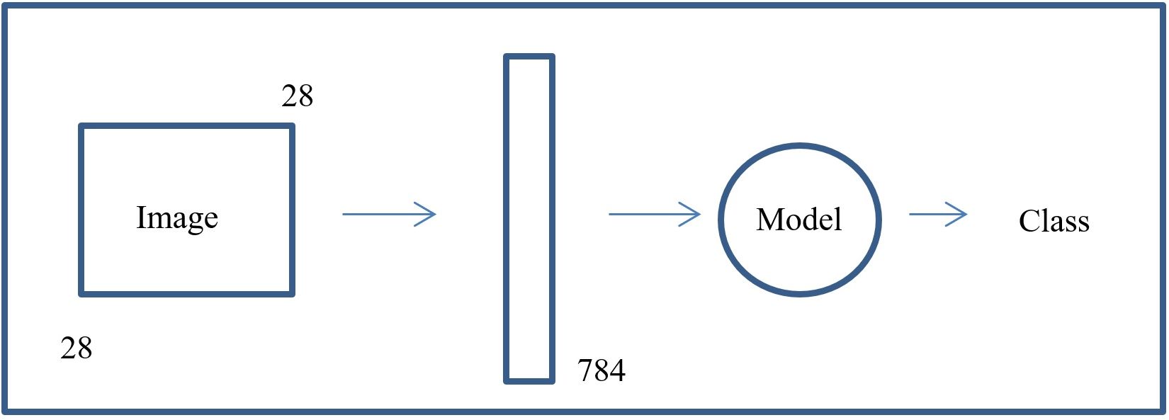
For the first example provided in this chapter, I will use the Mnist dataset. The goal of the RNN will be to classify the images into one of the 10 classes. In previous chapters, we have treated each image as a sample static in time of size 28x28 that we want to classify as a digit. In the RNN, we still want to classify each image into one of the 10 digits. However, in the RNN we will not treat each image as a vector of 784 features or tensor of size 28x28. Instead, we will use a sequence modeling approach to classify the image. So, to summarize, let us compare the RNN’s approach to previous approaches. In previous approaches we looked at the whole image as an instance of 784 features or tensor of 28x28 and classified it that way. The figure below shows the non-sequential pipeline.

With the RNN we look at each image as a sequence of segments of the image or patches (e.g. a sequence in time). We use this sequence from beginning to end to predict the final class for the image. With RNNs the pipeline is as follows:

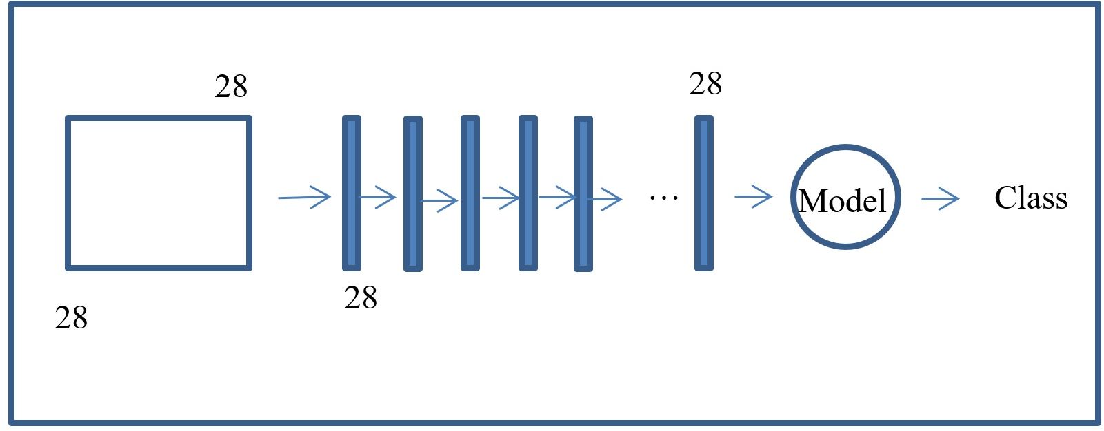
So, it can be seen in the previous image that the 28X28 image is converted into 28 vectors of 28 features each (the pixels). These vectors are fed sequentially into the model. With this definition of how to represent the input data, we can proceed to define the RNN algorithm. When I build NN models, I like to build simple networks first with random data to figure out the tensor dimensions. Once I understand the tensor multiplications and dimensions, I then feel ready to implement the architecture and train the model. So, in this section I will show this process. First, I will run the simplest torch RNN module on some dummy data. After that, we can proceed at building the RNN model for MNIST. Let us define the libraries here to get them out of the way. The only new steps will be to invoke the rnn modules from PyTorch. These modules will help us to define the architecture.

import torch import numpy as np import os from torchvision import datasets from torchvision import transforms import matplotlib.pyplot as plt import pandas as pd from numpy import genfromtxt from PIL import Image import sklearn from sklearn.metrics import confusion_matrix from sklearn.metrics import precision_score, recall_score, accuracy_score, f1_score from mlxtend.plotting import heatmap from sklearn.model_selection import train_test_split from torch.utils.data import TensorDataset, DataLoader import torch.optim as optim import torch.nn as nn import torch.nn.functional as F from torch.autograd import Variable

Reshaping Tensors for use with RNNs and dummy data

First, let us initialize the the RNN module. The basic RNN requires [vector_size, hidden_size, n_layers]. As can be seen in the following code segment:

## (vector_size, hidden_size, n_layers) rnn_basic_rc = nn.RNN( 10, 20, 2)

The parameters can be visualized in the following graph:

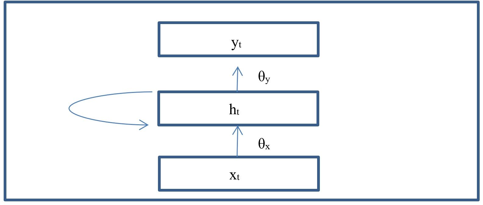
In the previous graph, the parameter "vector_size" refers to size of "x_t". It indicates the number of features in that vector. For the MNIST, it represents the rows in the image which are of size 28 at time "t". The parameter "hidden_size" refers to the number of neurons in the hidden layer "h_t". And finally, the variable "n_layers" refers to the number of hidden layers. In this case the recurring line going from "h_t" back onto itself.
Next we can create the dummy data.

## This is the data ## 28, 1000, 28) ## ( seq_len, batch_size, vector_size) input_basic_rnn = torch.randn( 5, 3, 10) input_basic_rnn.shape

Notice the shape of the data. We are used to seeing the shape of MNIST to be [number of batches, 28, 28]. However, traditionally RNNs have expected the data to look like this [28, number of batches, 28]. So remember to always reshape your data. Torch already makes this step not necessary. But I continue to use it to force myself to pay more attention to what I am doing when using RNNs. Here, the first 28 dimension is for the sequence length and the last 28 dimension is for the size of vector.
We now proceed to run the data through the RNN as can be seen here

output_zz, hn = rnn_basic_rc(input_basic_rnn, h0)

The RNN needs values for the hidden layer at time "t" equal zero since that is the first hidden layer in the sequence. That is usually solved by initializing that first hidden layer to random or zero values. This can be seen in the next code segment.

## (n_layers, batch_size, hidden_size) h0 = torch.randn( 2, 3, 20) h0.shape ## [2, 3, 20])

Finally, printing the shapes of "output_zz" and "hn" gives us [5, 3, 20] and [2, 3, 20], respectively. In the next section we will repeat this exercise but with the dimensions for the MNIST dataset.

Classifying MNIST with RNNs

In this section, we will focus on training an RNN for MNIST classification. First we will try using some dummy data just to look at the dimensions. After that, we can proceed to train the actual RNN model on the real MNIST data.

Visualising the dimensions of MNSIT for the RNN

Let us start by setting a size for the number of batches such as

N_batches_rc = 100

Now we create a batch of dummy data with the MNSIT dimensions. This can be done as follows:

## xb shape (batch_size, seq_len, vector_size) xb_rc = torch.randn(N_batches_rc, 28, 28) xb_rc.shape

This data needs to be permuted since the RNN traditionally has wanted data like this [28, number of batches, 28]. We do that with the following code segment

xb_rc = xb_rc.permute(1, 0, 2) xb_rc.shape ## [28, 100, 28]

As previously described, we now need to initialize the first hidden layer "h_0". We do that as follows:

## hidden has shape (n_layers , batch_size, rnn_hidden_size) ## ( n_layers, batch_size, rnn_hidden_size) hidden_rc = torch.zeros( 1, N_batches_rc, 128) hidden_rc.shape ## [1, 100, 128]

We are now ready to initialize the RNN and run the data through it as can be seen here

rnn_rc = nn.RNN( 28, 128, 1) rnn_o, hidden_rc = rnn_rc(xb_rc, hidden_rc ) print(rnn_o.shape) ## [28, 100, 128]

By definition, the RNN returns 2 parameters. The parameter "hidden_rc" will contain the last hidden embedding of size 128 at time "t=28" for every image in the batch. This can be run through a fully connected layer that takes the embedding of size 128 and converts to the output vector of size 10. This will hold the predicted class which can be compared to the real class.
Let us define the fully connected layer and run the last hidden layer as follows

fully_connected_rc = nn.Linear(128, 10) out = fully_connected_rc( hidden_rc ) ## [1, 100, 10] y_pred = out.view(-1, 10) # batch_size X n_output for 10 classes print( y_pred.shape ) ## [100, 10]

As can be seen, our predicted classes for every image in the batch (100 images) will be contained in "y_pred". That completes this discussion. We are now ready to train the RNN on the real MNIST data.

The RNN code for MNIST

As previously indicated, to predict the class per each 28x28 image we now think of the image as a sequence of rows. Therefore, you have 28 rows of 28 pixels each and we need to define this using some parameters. In this case, each row will be defined as a chunk or vector and the size of each chunk or vector will be defined as the chunk size (vector size). So we end up with a chunk_size = 28, a number of chunks of n_chunks = 28 (sequence length). We still have the standard set of 10 classes. We define that as n_classes = 10. Finally, the architecture will require us to define the size of the RNN hidden layer. We do that with rnn_size = 128. Let us define these parameters as follows:

learning_rate = 0.003 ## Adam default batch_size = 1000 ## 100 N_Epochs = 20 ##27000 seq_len = 28 # MNIST data input (img shape: 28*28) size_of_vector = 28 # chunks per image rnn_hidden_size = 128 # size of rnn n_classes = 10 # MNIST total classes (0-9 digits)

After defining the parameters, the next step is to load the data. As can be seen below, this step is exactly like previous steps.

data_path = "data/MNISTdata/" mnist_train = datasets.MNIST(data_path, train=True, download=True) mnist_test = datasets.MNIST(data_path, train=False, download=True) mnist_train_tr = datasets.MNIST(data_path, train=True, download=False, transform=transforms.Compose([ transforms.ToTensor() ])) mnist_test_tr = datasets.MNIST(data_path, train=False, download=False, transform=transforms.Compose([ transforms.ToTensor() ]))

It is always a good idea to print the tensor shapes before creating the data loaders.

data_path = "data/MNISTdata/" mnist_train = datasets.MNIST(data_path, train=True, download=True) mnist_test = datasets.MNIST(data_path, train=False, download=True) mnist_train_tr = datasets.MNIST(data_path, train=True, download=False, transform=transforms.Compose([ transforms.ToTensor() ])) mnist_test_tr = datasets.MNIST(data_path, train=False, download=False, transform=transforms.Compose([ transforms.ToTensor() ]))

For the shapes

mnist_train_tr.data.shape ## [60000, 28, 28] mnist_test_tr.data.shape ## [10000, 28, 28] train_dl = torch.utils.data.DataLoader(mnist_train_tr, batch_size=batch_size, shuffle=True ) test_dl = torch.utils.data.DataLoader(mnist_test_tr, batch_size=batch_size, shuffle=False )

As previously discussed we need to convert data from the format [batch size, 28, 28] to the shape [28, batch size, 28]. We will do this with the following function.

## MNIST data input (img shape: 28*28) ## seq_len = 28 ## size_of_vector = 28 ## batch_size ## Permute converts to [seq_len=28, batch_size, size_of_vector=28] def make_img_to_sequence(batch_x): batch_x_new = batch_x.permute(1, 0, 2) return batch_x_new

We can visualize the data as a batch of sequences below. Each row represents an image of 28 chunks with 28 features each sequence.

xb = [ 1, 2, 3, ..., 28 [ [1,2,3,...,28], [1,2,3,...,28], [1,2,3,...,28], ..., [1,2,3,...,28] ] [ [1,2,3,...,28], [1,2,3,...,28], [1,2,3,...,28], ..., [1,2,3,...,28] ] [ [1,2,3,...,28], [1,2,3,...,28], [1,2,3,...,28], ..., [1,2,3,...,28] ] [ [1,2,3,...,28], [1,2,3,...,28], [1,2,3,...,28], ..., [1,2,3,...,28] ] ... [ [1,2,3,...,28], [1,2,3,...,28], [1,2,3,...,28], ..., [1,2,3,...,28] ] ]

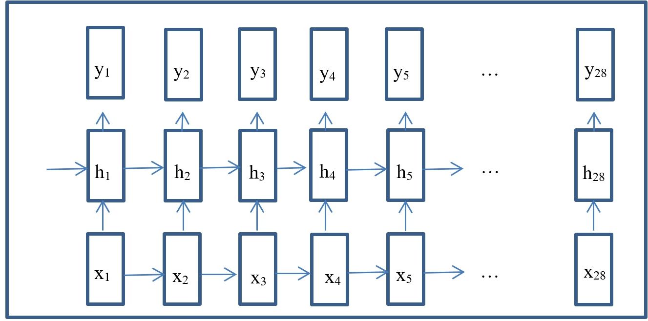
And just like that we are ready to define the RNN architecture. Generally speaking, an RNN can be thought of as a regular neural network except that it now has the additional behavior of recurrence per time step and also has a sequence of input. This recurring hidden layers can be represented as follows:

The architecture of an RNN can be expressed with the following equations.
$ y_{t} = \theta_y \phi(h_t)$
where $h_t$ can be defined as follows:
$ h_{t} = \theta_h \phi(h_{t-1}) + \theta_x x_t$
In diagram form, the equations can be represented as follows

The RNN architecture is defined in the next code segment.

## rnn_hidden_size = 128 # size of rnn hidden layer ## n_classes = 10 # MNIST total classes (0-9 digits) class MNIST_RNN_Net(nn.Module): def __init__(self): super().__init__() self.n_layers = 1 ## number of hidden layers self.hidden_dim = 128 self.seq_len = 28 self.size_of_vector = 28 ## (size_of_vector, rnn_hidden_size, n_layers) self.rnn1 = nn.RNN( 28, 128, 1) self.dropout = nn.Dropout(0.2) self.fully_connected = nn.Linear(128, 10) def init_hidden(self,): ## Initial hidden layer in time is all zeros ## (n_layers, batch_size, rnn_hidden_size) return torch.zeros( 1, batch_size, 128) def forward(self, xb): batch_x_seq = make_img_to_sequence( xb ) self.hidden = self.init_hidden() ## the initial hidden state ## self.hidden now contains the final hidden state ## for each image in the batch rnn_o, self.hidden = self.rnn1(batch_x_seq, self.hidden) rnn_o = self.dropout(rnn_o) out = self.fully_connected(self.hidden) ## batch_size, n_classes) y_pred = out.view( -1, 10) return y_pred

We will need to make a change to the training function as can be seen below. The function is very much the same as before except for the following line

xb = torch.squeeze(xb, dim=1)
Notice that this line reshapes the batch tensor from [1000, 1, 28, 28] to [1000, 28, 28]. The torch DataLoaders by default add the channel dimension but here we need to remove it.

def training_loop( N_Epochs, model, loss_fn, opt ): for epoch in range(N_Epochs): for xb, yb in train_dl: xb = torch.squeeze(xb, dim=1) y_pred = model( xb ) loss = loss_fn(y_pred, yb) opt.zero_grad() loss.backward() opt.step() if epoch % 1 == 0: print(epoch, "loss=", loss)

And that is it. We can now train the model by calling the core functions

model = MNIST_RNN_Net() loss_fn = nn.CrossEntropyLoss( ) opt = torch.optim.Adam( model.parameters(), lr=learning_rate ) training_loop( N_Epochs, model, loss_fn, opt )

and we can see the losses as follows

0 loss= tensor(0.7966, grad_fn=<NllLossBackward0>) 1 loss= tensor(0.5190, grad_fn=<NllLossBackward0>) 2 loss= tensor(0.3908, grad_fn=<NllLossBackward0>) 3 loss= tensor(0.3493, grad_fn=<NllLossBackward0>) 4 loss= tensor(0.2222, grad_fn=<NllLossBackward0>) 5 loss= tensor(0.2323, grad_fn=<NllLossBackward0>) 6 loss= tensor(0.1736, grad_fn=<NllLossBackward0>) 7 loss= tensor(0.1896, grad_fn=<NllLossBackward0>) 8 loss= tensor(0.1853, grad_fn=<NllLossBackward0>) 9 loss= tensor(0.1508, grad_fn=<NllLossBackward0>) 10 loss= tensor(0.2498, grad_fn=<NllLossBackward0>) 11 loss= tensor(0.1576, grad_fn=<NllLossBackward0>) 12 loss= tensor(0.1109, grad_fn=<NllLossBackward0>) 13 loss= tensor(0.1599, grad_fn=<NllLossBackward0>) 14 loss= tensor(0.1040, grad_fn=<NllLossBackward0>) 15 loss= tensor(0.1183, grad_fn=<NllLossBackward0>) 16 loss= tensor(0.1157, grad_fn=<NllLossBackward0>) 17 loss= tensor(0.0969, grad_fn=<NllLossBackward0>) 18 loss= tensor(0.0790, grad_fn=<NllLossBackward0>) 19 loss= tensor(0.1113, grad_fn=<NllLossBackward0>)

From the losses, we can infer that the model is learning. After training, we proceed to evaluate on the test set

f1_scores_to_plot = [] with torch.no_grad(): for xb, yb in test_dl: xb = torch.squeeze(xb, dim=1) y_pred = model( xb ) vals, indeces = torch.max( y_pred, dim=1 ) preds = indeces f1, last_conf_mtrx = print_metrics_function(yb, preds) f1_scores_to_plot.append(f1)

The results look really good (for a batch of 1000 test samples) and our RNN model has learned to classify the images.

Confusion Matrix: [[100 0 0 0 0 2 0 0 0 0] [ 0 118 0 0 1 0 0 0 0 0] [ 2 0 85 2 0 2 0 2 5 1] [ 0 0 0 101 0 0 0 0 0 1] [ 0 0 0 0 91 0 0 1 0 0] [ 3 0 0 0 0 81 1 0 0 0] [ 0 0 0 0 0 2 100 0 0 0] [ 0 0 3 0 0 0 0 112 0 0] [ 0 0 0 0 0 1 0 0 93 0] [ 0 0 0 0 1 0 0 1 0 88]] Precision: 0.969 Recall: 0.969 F1-mesure: 0.969

Summary

In this chapter Recurrent Neural Networks (RNNs) were presented and discussed. An example using the Mnist hand written digits data set was used for the analysis. Issues related to data representation and RNN architecture were also discussed.