Chapter 9 - Reinforcement Learning

In this section of the book I will cover the topic of Reinforcement Learning. This is an area of machine learning somewhere between supervised learning and unsupervised learning. It has been extensively applied to recommender systems and AI-based games. Recently, it was shown that a deep Q-network, using only pixels and game scores as inputs, could achieve a playing level comparable to that of professional human gamers across a set of 49 Atari games (\babelEN{\cite{mnihRef}}). The main advantage of applying reinforcement learning to games is that games are governed by rules. You have game states (the inputs) and actions (output) that lead to new states and rewards (the objectives to maximize). Because of this, no annotation is needed and instead you rely on the rules of the game for feedback (e.g. instead of annotated labels).

Copyright and License

Copyright © by Ricardo A. Calix.
All rights reserved. No part of this work may be reproduced or transmitted in any form or by any means, without written permission of the copyright owner.
MIT License.

FTC and Amazon Disclaimer

This post/page/article includes Amazon Affiliate links to products. This site receives income if you purchase through these links. This income helps support content such as this one.

Reinforcement Learning

In this section of the book I will cover the topic of Reinforcement Learning. This is an area of machine learning somewhere between supervised learning and unsupervised learning. It has been extensively applied to recommender systems and AI-based games. Recently, it was shown that a deep Q-network, using only pixels and game scores as inputs, could achieve a playing level comparable to that of professional human gamers across a set of 49 Atari games (\babelEN{\cite{mnihRef}}). The main advantage of applying reinforcement learning to games is that games are governed by rules. You have game states (the inputs) and actions (output) that lead to new states and rewards (the objectives to maximize). Because of this, no annotation is needed and instead you rely on the rules of the game for feedback (e.g. instead of annotated labels). There are several types of reinforcement learning techniques. In this chapter, I will focus on getting started with Q-learning since this is the technique used in the Mnih et al (2015) paper I referenced above. Here, I will try to provide a simple intuition based description of the technique. I should note that to achieve the level of Q-Learning presented in the Mnih et al (2015) paper, several additional optimizations need to be included. However, the discussion in this chapter should provide a simple way to get started with Q-Learning.

So what is Q-Learning?

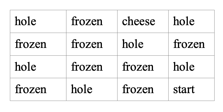
Q-Learning tries to learn the value of being in a given state (s), and taking a specific action from there. As I indicated, Q-learn has been applied to games. The best way to understand the algorithm is to analyze it from the point of view of a game. Here we will use Python’s OpenAI Gym module to play games. We will select the simple FrozenLake game environment. FrozenLake is a game about crossing a frozen lake that has some cracks in the ice with holes and there is wind sometimes that pushes the person crossing it. The game is very simple and consists of a grid that is 4x4 like so.

So, the objective is to get to the cheese without falling into a hole or being pushed by the wind into a hole. There are 4 moves which are up, down, right, and left. There is only one reward and that is to get to the cheese. However, you only get that reward in the future by first taking several steps on frozen blocks without falling in a hole. Therefore, one challenge is that you have to state your objective in terms of several future moves. This is accomplished using something called the Bellman Equation. The key to predicting these rewards is to know the associated reward given a current state and action to take. This is called a Q mapping

Q (state, action) = reward

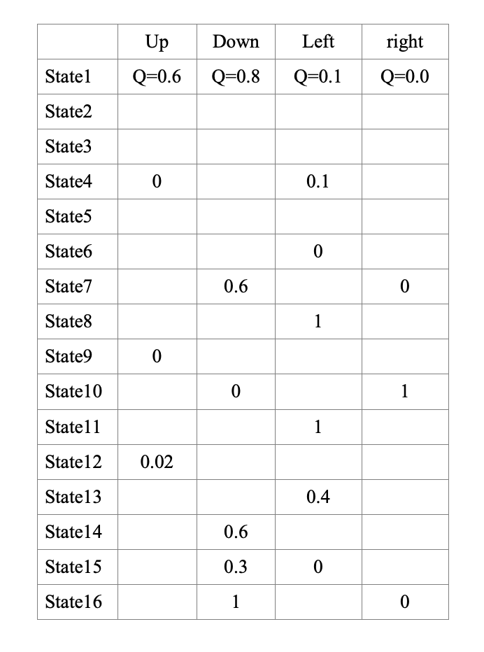
For such a simple grid, we could just use a table. In this case our table would be 16x4 because there are 16 possible states (position in the grid of 4x4) and there are 4 actions (up, down, right, left). Since we know the rules of the game and the layout of the grid, we can populate the table and learn the Q rewards for each state/action pair. An example of the table can be seen below.

Now the main challenge is that we need to learn future rewards for future actions as we move through the grid. Here the Bellman equation will help. Think of the Bellman equation as a type of recursive equation that looks at the future state given a current state. The Bellman equation is as follows:

Q(state, action) = reward + weight * max [ Q(future_state, future_action ) ]

These values can be looked up from the Table. The code discussed here can be downloaded from the course website or the github repository. In the next section, the python Q-learning code will be discussed which only uses a table to determine the rewards and the path to follow. Future sections will use the same algorithm but will replace the use of the table with a neural network so that we can see how deep neural networks can improve the approach.

Q-Learning using a Table

In this section we discuss the code to implement Q-Learning using a table. This code makes use of the OpenAI gym library. The libraries used can be seen in the next code segment.

import numpy as np import gym

The frozenLake game can be initialized by creating the env object as can be seen below. This object represents the game and holds all the parameters related to states, actions, rewards, and current game state.

env = gym.make('FrozenLake-v0')

The next step is to initialize the table $ Q $ to all zeros and of size 16x4. Here env.observation\_space.n = 16 and env.action\_space.n = 4.

Q = np.zeros( [env.observation_space.n, env.action_space.n] ) lr = 0.8 y = 0.95 num_episodes = 2000

We take 2000 epochs (or episodes) and initialize some parameters lr and y. Each episode represents a game played. We use \textbf{jList} and \textbf{rList} to collect the number of steps taken per episode and the total reward per episode, respectively. These are used to collect results of each game.

jList = [] rList = []

The following code segment goes over the main loop of the Q-learn algorithm.

for i in range(num_episodes): s = env.reset() rAll = 0 d = False j=0 while j < 99: j+=1 zz = env.action_space.n a=np.argmax(Q[s,:]+np.random.randn(1,zz) *(1.0/(i+1))) s1,r,d,_ = env.step(a) Q[s,a] = Q[s,a] + lr*(r + y*np.max(Q[s1,:]) - Q[s,a]) rAll += r s = s1 if d == True: break #jList.append(j) rList.append(rAll)

In the next code segment, the line

for i in range(num\_episodes):

indicates that we are going to play num\_episodes = 2000 games. During these 2000 tries we will learn the best path to take. From the main loop we can see that the line

s = env.reset()

restarts the game for every episode so we can play it again and assign the initial state to \textbf{s}. The variable \textbf{rAll} adds up the accumulated rewards for this episode. The variables \textbf{d} and \textbf{j} are control variables to indicate if the game has ended and to count the number of steps taken. The code in the while loop is what allows the algorithm to learn or update the values in the \textbf{Q} table designated by the variable \textbf{Q}. To take the first step we need to pick an action to follow. We do this with the following lines of code:

zz = env.action_space.n

and

a = np.argmax( Q[s,:]+np.random.randn(1,zz) *(1.0/(i+1)) )

The variable \textbf{zz} is the size \textbf{n} of all actions in the game (up, down, left, right) which in this case is 4. The statement Q[s, :] selects the current Q values (rewards) associated with state \textbf{s}. The statement

np.random.randn(1,zz) *(1.0/(i+1))

adds randomness to the four Q values for the current state. Basically, you randomly increment the Q values for the current state and then select the highest one with

np.argmax()

by selecting the highest Q value you determine what action (a) you take given the current state. Once the action "a" is selected, we can proceed to evaluate it in the game to obtain our new state (position) and the reward (did we fall in a hole or advanced to a frozen block). We do this with

s1, r, d, _ = env.step(a)

here, "s1" is the new state (position) and \textbf{r} is the reward. The parameter \textbf{d} indicates end of the game. Given this new information about the result of our action, we can proceed to update the Q-table with our new results and new knowledge about the state of the game. This is done with the statement

Q[s,a] = Q[s,a] + lr*(r + y*np.max(Q[s1,:]) - Q[s,a])

In this statement, \textbf{Q[s, a]} contains the current Q value (reward) associated with the state \textbf{s} and the action \textbf{a}. This is the Bellman equation which can be viewed as

next_s_Q = lr*(r + y*np.max(Q[s1,:]) - Q[s,a])
Q[s,a] = Q[s,a] + next_s_Q

The term next_s_Q contains the current reward for state \textbf{s} plus the maximum reward for the next state \textbf{s1}. The parameters \textbf{lr} and \textbf{y} are weights to control the importance of the next state’s reward when updating the current states reward (Q value). We can think of this parameter

- Q[s,a] )

as a regularization parameter. At this point we are almost done and we can proceed to accumulate our results. The statement

rAll += r

accumulates the total rewards. The statement

s = s1

assigns the current state \textbf{s1} to \textbf{s}. The "if" statement in the folowing code listing

if d == True: break

ends the game if \textbf{d} indicates end of game. The statement

jList.append(j)

accumulates the number of steps taken to reach end of game. The statement

rList.append(rAll)

appends rewards per game to a list so that they can be viewed later. That is it. We have finished our discussion of Q-learn with tables on the frozenLake game. Now we can proceed to replace the table with a neural network.

Q-Learning using a Neural Network

Now that we understand the frozenLake game with a table, we can proceed to replace the table with a neural network. It is important to note here that the weights matrix \textbf{W} in the neural network can be thought of as representing the \textbf{Q} table. Otherwise, just think of the whole neural network as the table. We give it the states vector (size=16) as input and the network predicts the actions vector (size=4) per state. Let us begin.
First we include the libraries as can be seen below. Notice we now add PyTorch.

import gym import numpy as np import random import torch import matplotlib.pyplot as plt import torch.nn as nn import torch.nn.functional as F import torch.optim as optim

We create the game with the env object.

env = gym.make('FrozenLake-v1')

Next, we define our familiar neural network classes and functions for the loss and training. The first Q NN class creates a simple logistic regression type neural network. Here, the \textbf{W} replaces the \textbf{Q} table. Notice the dimensions of \textbf{W} are 16x4 because we have 16 states in the game and 4 actions. The \textbf{Qout} tensor (our predicted \textbf{y} in previous chapters) is the result of a matmul operation between \textbf{x} (our states) and \textbf{W} (the weights or Q values in this case).

class Q_NN_Net(nn.Module): def __init__(self): super().__init__() self.linear1 = nn.Linear(16, 4) self.act1 = nn.Softmax(dim=1) def forward(self, s): x = gen_state_vector(s) x = self.linear1( x ) Qout = self.act1( x ) Qout = torch.squeeze(Qout, 0) return Qout

With

torch.squeeze(Qout, 0)

we get the actions vector. We will use a torch.max function later to select the action. As can be seen from the previous class code, the network looks like the figure below.

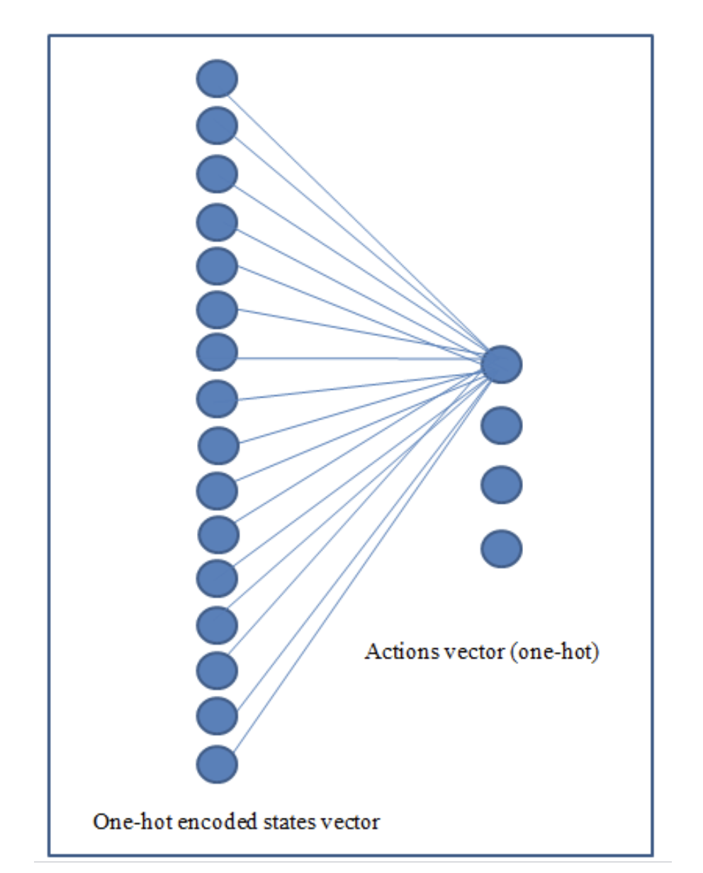
It is important to note that this is a basic architecture and that much more complex deep architectures with different activation functions could be used such as architectures with many hidden layers or convolutional neural networks, etc. I was able to achieve good results using the following MLP neural network architecture.

class Q_NN_MLP_Net(nn.Module): def __init__(self): super().__init__() self.linear1 = nn.Linear(16, 10) self.act1 = nn.ReLU() ## Tanh() ## nn.Sigmoid() self.linear2 = nn.Linear(10, 4) self.act2 = nn.Softmax(dim=1) def forward(self, s): x = gen_state_vector(s) x = self.linear1( x ) x = self.act1( x ) x = self.linear2( x ) Qout = self.act2( x ) Qout = torch.squeeze(Qout, 0) return Qout

Notice that the NN classes us the following function called \textbf{gen\_state\_vector(s)}. We will use this function to convert state in integer form into one hot encoded vectors of size 16.

def gen_state_vector(s): states_np = np.identity(16)[s:s+1] states_np = states_np.astype( np.float32 ) ## print(states_np.dtype ) inputs1 = torch.from_numpy( states_np ) return inputs1

The function

gen_state_vector(s)

takes the current state in the variable \textbf{s} and converts it into a one-hot encoded representation. For instance, if the current state is 4, then the one-hot encoded representation (of size 16) looks like this

[0, 0, 0, 1, 0, 0, 0, 0, 0, 0, 0, 0, 0, 0, 0, 0]

The loss function can be Least Squares Estimation which is the same as for regression! To calculate the error, we basically compare \textbf{q_pred} to \textbf{target_q} and try to minimize the error.

loss = F.smooth_l1_loss( q_pred, target_q ) ## or loss_fn = nn.MSELoss()

We can set the following parameters. We create lists to contain steps taken per episode (game) and rewards per game.

stepsList = [] rewardsList = [] success_list = [0.0005] learning_rate = 0.001 ## Adam default learning rate y = 0.99 num_episodes = 4000 epsilon = 0.1 ## 0.2 , 0.01

The optimization is nothing more than the very familiar Gradient Descent (Adam) with a learning rate of 0.001. We instantiate the Q NN MLP model.

## model = Q_NN_Net() model = Q_NN_MLP_Net() opt = torch.optim.Adam( model.parameters(), lr=learning_rate )

Finally, we are ready for the main loop which is shown in the next code segment below.

for i in range(num_episodes): s = env.reset() s = s[0] ## env returns tuple so select first of tuple rAll = 0 d = False j = 0 if i % 200 == 0: print("Game ", i, " of ", num_episodes) while j < 1000: Q_s = model( s ).detach() _, max_index = torch.max(Q_s, 0) a = max_index.item() s1, r, d, _, _ = env.step(a) if d == True and r == 0: r = -1 Q_s1 = model( s1 ).detach() # detach from graph maxQ_s1 = torch.max( Q_s1 ) target_q = r + 0.99 * maxQ_s1 q_pred = model( s )[a] ## loss = loss_fn( q_pred, target_q ) loss = F.smooth_l1_loss( q_pred, target_q ) opt.zero_grad() loss.backward() opt.step() rAll = rAll + r j = j + 1 s = s1 if d == True: break if d == True and r > 0: success_list.append(1) stepsList.append(j) ## steps taken per game else: success_list.append(0) ## stepsList.append(j) ## steps taken per game rewardsList.append(rAll) ## reward total per game

I will now proceed to break the main loop into parts to make it easier to describe. As can be seen in the code segment below, we run the main loop 4000 times (\textbf{num_episodes}) which means that we play 4000 games. Each time we play a game, we reinitialize the board ( s = env.reset() ) and initialize the rewards variable (\textbf{rAll}) to zero. The variable \textbf{j} is the counter for the current step and \textbf{d} is used to determine if the game is over (win or loss).

for i in range(num_episodes): s = env.reset() s = s[0] ## env returns tuple so select first of tuple rAll = 0 d = False j = 0 if i % 200 == 0: print("Game ", i, " of ", num_episodes)

for every game iteration we run the following while loop. This while loop is the main code that helps us to learn the \textbf{Q} values and traverse the board (e.g. play the frozen lake game).

while j < 1000: Q_s = model( s ).detach() _, max_index = torch.max(Q_s, 0) a = max_index.item() s1, r, d, _, _ = env.step(a) if d == True and r == 0: r = -1 Q_s1 = model( s1 ).detach() # detach from graph maxQ_s1 = torch.max( Q_s1 ) target_q = r + 0.99 * maxQ_s1 q_pred = model( s )[a] ## loss = loss_fn( q_pred, target_q ) loss = F.smooth_l1_loss( q_pred, target_q ) opt.zero_grad() loss.backward() opt.step() rAll = rAll + r j = j + 1 s = s1 if d == True: break

We perform 1000 steps since it should not take more than 1000 steps to traverse the frozen lake. If it does, the game should end. The line in the while loop is used to increment the steps

j = j + 1

After incrementing the steps, we proceed to perform our first model run to train the PyTorch model. Here we predict an action and get Q_s from the model.

Q_s = model( s ).detach() _, max_index = torch.max(Q_s, 0) a = max_index.item()

The next step is to take the predicted action in \textbf{“a”} and run it through the game. The below statement runs the action through env.step() and this function returns the new state \textbf{s1} which is the new position in the frozen lake grid, \textbf{r} is the reward associated with the step \textbf{s} (for instance r = 0.43) , and \textbf{d} indicates if the game is over (found the cheese or fell in the frozen lake). You know you have lost the game if \textbf{d} is True and if the reward is zero at the same time. To help the model learn, we can assign negative rewards every time that happens. Knowing when to assign rewards is very challenging in Reinforcement Learning. Here, frozen lake is a simple game and using this type of approach is possible. Current research proposes to replace the rewards heuristics with neural networks. One current effective approach is called RLHF which stands for reinforcement learning through human feed-backs.

s1, r, d, _, _ = env.step(a) if d == True and r == 0: r = -1

With the new state \textbf{s1}, we proceed to run the PyTorch model again. Here we run the model again using \textbf{s1}.

Q_s1 = model( s1 ).detach() # detach from graph _, maxQ_s1 = torch.max( Q_s1 ) target_q = r + 0.99 * maxQ_s1

So \textbf{Q\_s1} will now contain the 4 neuron vector with the \textbf{Q} values for all 4 actions given state \textbf{s1}. We grab the max value from \textbf{Q\_s1} (not the index) and use that to calculate \textbf{target\_q} using the Bellman equation.
Recall that the Bellman equation looks like this:

Q(state, action) = reward + weight * max [ Q(future_state, future_action )]

Interestingly, only one of the 4 values in \textbf{Q\_s1} is updated using the Bellman equation. The other values remain the same. The dimension of \textbf{target\_q} is only one which means that that is the only value we will use to perform the optimization. Finally, we do a final update of the PyTorch model by calculating the losses on state \textbf{“s”} and action \textbf{a}.

q_pred = model( s )[a] ## loss = loss_fn( q_pred, target_q ) loss = F.smooth_l1_loss( q_pred, target_q ) opt.zero_grad() loss.backward() opt.step()

Finally, the last peace of code adds up the rewards, assigns the new state \textbf{s1} to \textbf{s}, and checks to see if the game is over.

rAll = rAll + r j = j + 1 s = s1 if d == True: break

Once you exit the while loop, the last part is to append the results of the current game to the results lists.

if d == True and r > 0: success_list.append(1) stepsList.append(j) ## steps taken per game else: success_list.append(0) ## stepsList.append(j) ## steps taken per game rewardsList.append(rAll) ## reward total per game

Well, that is it for the algorithm discussion. Finally, we print our results and plot them.

print("Percent of succesful episodes: " , str( sum(rewardsList)/ num_episodes ), "%") plt.plot(rewardsList) plt.show() plt.plot(stepsList) plt.show()

That is it. We have completed implementing our Q learning algorithm with a neural network. In the next section we will add a simple improvement to the code that will improve performance.

Performance, Q-NN, and randomness

In the previous section we described the code to implement Q-learning with a neural network on the frozen lake game. That was the simplest implementation of it.

for i in range(num_episodes): s = env.reset() s = s[0] ## env returns tuple so select first of tuple rAll = 0 d = False j = 0 if i % 200 == 0: print("Game ", i, " of ", num_episodes) while j < 1000: if (np.random.rand(1) < epsilon): a = env.action_space.sample() else: Q_s = model( s ).detach() _, max_index = torch.max(Q_s, 0) a = max_index.item() s1, r, d, _, _ = env.step(a) if d == True and r == 0: r = -1 Q_s1 = model( s1 ).detach() # detach from graph maxQ_s1 = torch.max( Q_s1 ) target_q = r + 0.99 * maxQ_s1 q_pred = model( s )[a] ## loss = loss_fn( q_pred, target_q ) loss = F.smooth_l1_loss( q_pred, target_q ) opt.zero_grad() loss.backward() opt.step() rAll = rAll + r j = j + 1 s = s1 if d == True: break epsilon = epsilon + epsilon_delta if d == True and r > 0: success_list.append(1) stepsList.append(j) ## steps taken per game else: success_list.append(0) ## stepsList.append(j) ## steps taken per game rewardsList.append(rAll) ## reward total per game

To improve the results, we can add a few lines of additional code which will allow the algorithm to better converge and learn better Q-values. The additions are simple and basically relate to adding randomness to the code. The full version of the code can be seen below. I will additionally discuss how to measure performance with RL.
The new lines of code add randomness to the selection of the next action to take. The idea is that at the beginning of the learning process, the action prediction function may not be very good. Therefore, picking an action randomly at the beginning may be better than picking actions with the model.
This is reflected in the code segment below.

if (np.random.rand(1) < epsilon): a = env.action_space.sample() else: Q_s = model( s ).detach() _, max_index = torch.max(Q_s, 0) a = max_index.item()

A random number is obtained and compared to \textbf{epsilon}. If less than \textbf{epsilon}, the action is selected randomly. As the algorithm improves and the Q values are better, the value of \textbf{epsilon} can be adjusted so that action is more often selected with the model and not with the random function.
The code can be seen here where the value of \textbf{“epsilon”} is adjusted.

epsilon = epsilon + epsilon_delta

That is all it takes to implement randomness. Now we are ready to measure the performance of the RL model using frozen lake. After training, we can perform several calculations to measure performance.
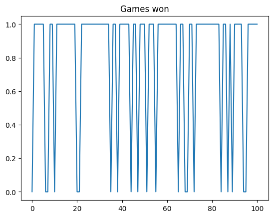
First let us count the number of successes during the last 100 training games (out of 4000). The following calculation gives us a score of 75\%.

print("Succes for last 100 games: ", sum(success_list[-100:]), "%")

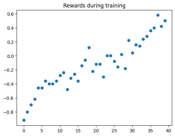
We can look at the rewards trend with the following code.

## rewardsList = rewardsList[-20:] step_size = 100 ## new_avg_per_n_entries r_rc = [ sum(rewardsList[i:i+step_size])/step_size for i in range(0, len(rewardsList), step_size ) ] rewardsList = r_rc print(rewardsList) print(set(rewardsList)) print(len(rewardsList)) print(sum(rewardsList)) print( num_episodes ) ind_rew = [i for i in range(len(rewardsList))] plt.scatter(ind_rew, rewardsList) ## plt.plot(rewardsList) plt.title("Rewards during training") plt.show()

During training, we collected the total reward per each of the 4000 games. Visualising all 4000 rewards can be confusing. However, if we average every 100 rewards in sequence, we can clearly see that the rewards are going up. One of the goals in RL is for the model to increase its rewards.

Once the model is trained, we want to run it again without training to test its performance. This can be accomplished with the following code

stepsList = [0.0005] success_list = [0.0005] test_games = 100 for i in range(test_games): s = env.reset() s = s[0] j = 0 while j < 1000: agent_out = model(s).detach() _, max_index = torch.max(agent_out, 0) a = max_index.data.cpu().numpy()[()] s1, r, d, _, _ = env.step(a) if d == True and r == 0: r = -1 s = s1 j = j + 1 if d == True: break if d == True and r > 0: success_list.append(1) else: success_list.append(0) stepsList.append(j)

After running the evaluation (no training), the model is able to win 79\% of the games it played.

Summary

In this chapter we have discussed the Q learning algorithm as part of the larger topic of Reinforcement Learning using tables and neural networks with randomization.